An FGS observer may find that a single observation requires a detailed investigation. As an example, a particular star in a Position mode observation that appears on one or more plate overlays with large, unexplained residuals, or if the acquisition of the star failed. STScI has developed several tools for analyzing individual observations using the raw GEIS files as input rather than the pipeline products (refer to Chapters 1 and 2 of this Handbook for instructions on retrieving data from the HST archive and for information on the GEIS file format). These tools include the interactive graphics package fgsplot which allows for a variety of FGS quantities to be plotted, the interactive ASCII display tool read-fgs, which displays the values of selected samples of raw data, and the tool export-fgs, which outputs the 40hz x and y position of the FGS’s instantaneous field of view (IFOV), the photomultiplier tube (PMT) counts, and the values of the FGS flags and status bits. Each of these will be discussed in the following sections.

Please note that a detailed discussion for the preparation and analysis of Transfer Mode observations, which are treated as individual observations, is provided in Section 1.3. This section addresses more generic tools that are applicable to any FGS observation.

4.2.1 FGSPLOT

The interactive graphics tool fgsplot can be used to display a variety of FGS quantities from the raw GEIS files. For example, the location of the IFOV in the FGS detector space coordinates can be displayed as a function of x vs. y, or the fine error signal (partial S-curve) as a function of x during the WalkDown to FineLock. The source code for fgsplot is available via download from the FGS Website (follow the link under tools). It is a mixture of Fortran and C using SM for the graphic displays.

The fgsplot tool is both versatile and essential for analyzing failed observations and retrieving useful data from marginal observations. The tool can also be a valuable educational aid for an observer who is unfamiliar with FGS data. An example terminal session using fgsplot is displayed on the following pages. The reader is encouraged to consult this example while reading about fgsplot.

The fgsplot tool is a package of Fortran and C modules that can be downloaded from the FGS Website. A Makefile and instructions are also available to facilitate the building of an executable image on a UNIX or LINUX based host.

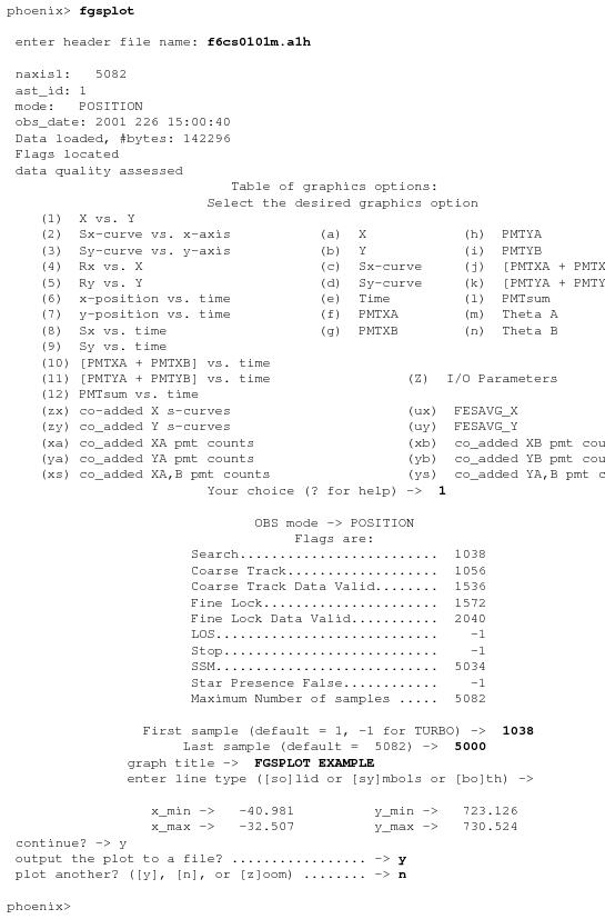
Once an executable image is constructed, the tool is activated by simply typing fgsplot.e (or its alias). At the prompt, enter the name of the data set’s header file (i.e., f2p30104m.a1h). fgsplot will open and read the header and data files and prompt for instructions as to what to plot. A menu is presented to facilitate the selection. The options come in two basic varieties. First is a set of options with either numerical digits or double characters. This class contains the most commonly invoked options, such as plotting x vs. y (option 1), or PMTSUM vs. time (option 12), or displaying the acquisition of (or failure to acquire) the fringes of a star in FineLock (options 2 and 3).

The second class of options, denoted by single character alphabetical choices, allows one to plot a variety of items against one another. To invoke this capability one must enter two letters (with no spaces in between) to specify the quantities to be plotted. For example, entering “ab” will plot x vs. y, which, incidentally, is equivalent to specifying a “1”.

After entering a choice of quantities to be plotted, fgsplot will prompt for the range, in sample numbers, of the data to be plotted. To help make the choice meaningful, fgsplot displays the sample number of when a particular flag or status bit became set or when an event occurred. (If plotting a Transfer Mode observation, please refer to the section “fgsplot for Transfer Mode”.) For example, if one wishes to plot the location of the IFOV (x vs. y) from the moment when the search for the target began until the completion of the FineLock acquisition, the numerical value (sample number) displayed for the initiation of “Search” should be specified as the first sample, and the sample number of “FineLock DataValid” should be entered as the last sample number to be plotted. Note that simply hitting <ret> at the prompt for “first sample” defaults to sample = 1 (plotting from the beginning of the observation), while hitting <ret> at the prompt for “last sample” defaults to “Maximum number of Samples”, i.e., plotting to the end of the observation.

With the range of the data specified, fgsplot prompts for a title to be used to annotate the graph, and requests instructions as to whether or not to plot the data with a solid line or symbols at the data points, or both. Simply hitting <ret> invokes a solid line plot.

Prior to plotting, fgsplot will compute the minimum and maximum values (along the abscissa and ordinate) of the items to be plotted, display these values, and offer the user the option to continue or not. Any response other than “N” or “n” will cause the plotting to occur, at which time a SM X11 window appears with the graph, and the user is offered the opportunity to have the plot saved to a postscript file named rootname.i, where rootname is the data set name (f2r30201m, e.g.), and “i” is the value of a counter that increments each time fgsplot outputs a postscript file in the current session (fgsplot retains no memory of usage in previous sessions).

Next, the user is offered the option to repeat the entire process or to “zoom” in on the currently displayed plot. If the zoom option is invoked (by entering “z” or “Z”), fgsplot requests the minimum and maximum values of the quantity along the abscissa to be plotted. Over this range of abscissa data the corresponding minimum and maximum values of the quantity along the ordinate are computed and displayed. The user has the option of resetting the full range (in effect scale) of the ordinate axis before plotting the data. The graph is displayed and the option to output to a postscript file is offered.

If the “zoom” option is not invoked, but rather a new plot is specified, the entire process is repeated (with the exception of specifying the header file name). If different quantities (e.g. the y-axis fine error signal instead the x-axis fine error signal), but the same range of samples are to be plotted, one can then enter “-1” (the Turbo option) when prompted to enter the first sample to be plotted.

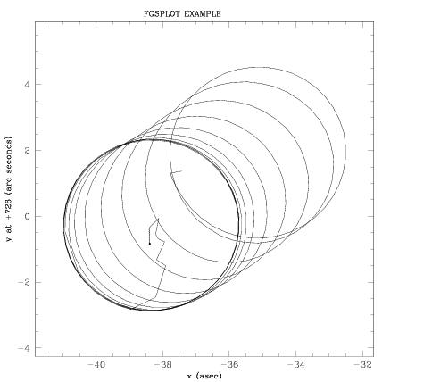
The data plotted in Figure 4.1 shows an example of the output from fgsplot. This plot shows the path of the FGS’s IFOV from the beginning of the search spiral, to Coarse Track, through the “walkdown” (acquisition) of FineLock, and finally the FineLock tracking of the star’s interferometric fringes. A terminal snapshot of a fgsplot session that produced this plot is shown on the following page. User inputs are denoted in bold.

fgsplot for Transfer Mode

Transfer Mode observations typically include many scans of the IFOV across the target, each generating an interferogram or S-curve. fgsplot offers the capability to co-add all or a selected subset of these scans and to plot data from the entire scan path or over a specified segment. Note, cross correlations and curve smoothing are not currently supported by fgsplot. This capability will be added by the fall of 2002. Check the FGS Website for updates.

fgsplot reads the header file to determine the data set’s observing mode (from the value of the keyword PASTMODE). If the data set is a Transfer Mode observation, fgsplot determines the number of scans that were executed, the length of the scans, and the start and end sample number of each scan. These results are displayed along with the sample number of the status flags and events listing (as discussed in the previous section) after the user specifies what quantities are to be plotted.

For choices that involve co-adding individual scans, such as “zx” or “zy”, fgsplot queries for the scans to be included in the co-addition. This can be specified either by explicitly entering the scan numbers (i.e. 1, 2, 3, 5, 10), or by specifying a range (i.e., 1-20, 25-50, which excludes scans 21 through 24). Simply hitting <ret> at the prompt causes all scans to be included in the co-addition.

For choices not involving co-addition, such as “1” (x vs. y), fgsplot prompts for the scan number whose start/end sample numbers identify the segment of the observation from which data are to be extracted for the plot. If the user enters <ret>, fgsplot reverts back to displaying the sample numbers for the various flags and events described earlier. The user then explicitly specifies the start/end sample number to define the interval from which data is extracted for plotting.

Finally, when scan IDs or co-added quantities are used to specify the start/end intervals from which data are extracted for plotting, fgsplot offers the option of plotting only a central segment of the scan, with a length specified by the user. Hitting <ret> at this prompt causes data along the entire scan length to be plotted.

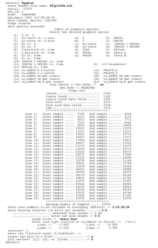
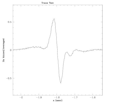
An example terminal session using fgsplot on a Transfer Mode observation is shown below (user input in bold). This observation contained thirty scans on a V=12 white dwarf (single) star. For illustration purposes, scans 1 through 10 and 21 through 30 were included in the co-addition of data along the X-axis, and only the central 0.5" of the full (0.85") scan path is plotted. The scans were binned with 2 mas intervals, and an output file of the resulting plot is requested, which is displayed in Figure 4.2. A reminder: this is a plot of raw data; cross correlation and smoothing are not supported by fgsplot. We plan to upgrade the package to support these tasks. Users are advised to check the FGS Website for updates.

Obtaining ASCII Output from fgsplot

fgsplot offers the option of creating an ASCII output file containing a two column listing of the data that is plotted. The number of rows will be equal to the number of data points in the plot. This can serve as a convenient method to quickly extract semi-processed data for additional quick look analysis or for input into more sophisticated graphics script (fgsplot offers very little support for annotation which might be desired for display and presentation purposes).

To obtain such an ASCII file one simply appends the choice designating the items to be plotted with an “*”. For example, entering “1*” (x vs. y) in response to the selection menu prompt produces a two-column ASCII file containing time-ordered X and Y values, with the number of entries exactly equal to the number of points plotted. Another example would be “zx*”, which generates an ASCII file with the x and the co-added x-axis interferogram.

The name fgsplot assigns to an ASCII file is determined from the header file’s rootname (i.e., f2d40203m) and a code that is used to specify what data are output. This code can be discerned from the selection menu of (single) items that can be plotted against one another. For example, if one specifies a plot of x vs. y by entering “ab*” at the selection prompt, then a file with the name “f2d40203m.fab” will be created. (Note that entering “1*” at the selection prompt, which is equivalent to specifying “ab*”, also generates a file named rootname.fab). If an output file is requested for options involving the co-addition of data, it will be named rootname.fxx, where xx = selected choice. For example, if an output file containing a listing of x vs. the co-added x-axis interferogram is desired, “zx*” is entered at the prompt, and the file “rootname.fzx” is created. Note that if the target output file already exists, fgsplot overwrites its contents, even within the same fgsplot session.

4.2.2 Read-FGS

The tool read-fgs reads FGS GEIS header and data files and displays selected contents of any of the 7 groups of data contained in the data file. The tool is a package of Fortran and C modules that can be downloaded from the FGS Website. A Makefile and instructions are also available to facilitate the building of an executable image on a UNIX or LINUX based host.

Once an executable image is constructed, the tool is activated by simply typing read-fgs.e (or its alias). read-fgs prompts the user for the name of the GEIS header file that is associated with the GEIS data file that is to be read. The appropriate header and data files are opened and read, and the user is prompted to specify the name of the group from which data is to be extracted and displayed. The option to type “h” for help is available to display the names of the groups, whose names and contents are displayed in Table 4.1.

Table 4.1: FGS Groups and Associated Data

To display data from the group PMTXA, simply type “pmtxa” at the prompt. The values of the first 32 samples from this group will be displayed in four columns. The option to display the next 32 samples, or to choose the starting sample number of the next 32 samples to be displayed is offered. Simply hitting <ret> defaults to displaying the next 32 samples. And, for example, typing 1000 will cause samples 1000 through 1031 to be displayed. If a number larger than NAXIS (the size of the group) is entered, the last 32 samples from the group are displayed.

To view the contents of a different group, enter either the group’s name or “q” at the prompt. If the group’s name is entered, the values of the first 32 samples are displayed. If “q” is entered, one is prompted to enter the name of the next group to be displayed. In either case, data from any location within the group can next be displayed as described in the paragraph above.

For illustration purposes, an example of a session with read-fgs is displayed below. User supplied input is in bold.

The flags group warrants special discussion. If this group is selected the user is prompted to choose whether the display is to be in ASCII or hex. The hex values are base16 displays of the 32 bit integers that comprise the flags group. The ASCII option invokes a translation of the values contained in these integers to display which flags or status bits are set (= 1). Flags that are not set (= 0) are not displayed. Table 2 lists the two character code used to represent a given flag or status bit. At any given time more than one flag is usually set. For example, when an FGS is tracking a star in FineLock (as in a Position mode observation), the flag display will be “SP,FL,DV”. Here “SP”, or Star Presence, indicates that the measured photometry from the star exceeds the minimum detection threshold, while “FL,DV” indicates that the star’s fringes have been successfully acquired and are being tracked in FineLock. Table 4.3 lists the sequence of values in the flags group for a typical FGS observation

Table 4.2: Two-character codes representing FGS flag or status bits

Table 4.3: Sequence of values in FGS flags

Two additional items will be encountered when one uses read-fgs. These are the values used for bad data and fill data, denoted by 999999 and 999998, respectively. The processor that extracts the FGS mnemonics from the engineering telemetry to build the GEIS files uses the bad data value when corrupt telemetry frames are encountered. The fill data value is used when the processor encounters missing frames, or, as in the case of the flags group, to pad the last 5/6 of the group. (The flags are sent only 1/6 as often as the other datums, but the flags group must be the same size as the others, so padding is required. This also implies, e.g., that flag group sample number 100 corresponds, in a temporal sense, to sample number 600 in the other groups). If bad data or fill data are encountered while the contents of the flags group is being viewed in ASCII mode, “bad data” or “fill data” is displayed.

The insertion of bad data or fill data indicators into the GEIS files preserves the temporal relation between samples. For example, sample number 100 records data that is (100-1)*25 msec. later than that recorded in sample number 1. This also preserves the mapping of data across groups. For example, the value of sample number 120 in group PMTXA was gathered at the same time as sample number 120 in all of the other groups (except flags, whose corresponding sample number would be 120/6 = 20).

4.2.3 Export-FGS

The tool export-fgs can be used to generate an ASCII version of the 6 header/data FGS GEIS files for a given observation. This might be useful if non-standard processing and analysis of an observation is desired. The tool can be downloaded from the FGS Website. Its source code is composed of Fortran and C modules. A Makefile and instructions on how to generate an executable image are also available.

To execute export-fgs simply type export-fgs.e or its alias from the directory containing the FGS GEIS files that are to be processed. At the prompt, enter the rootname of the data set to be processed. export-fgs will open and read the available GEIS files for each of the 3 FGS, and will create an ASCII file for each FGS. These files will each have 7 columns of data: x, y, pmtxa, pmtxb, pmtya, pmtyb, and the flags. The x, y values are computed from the star selector servo angles (ssenca and ssencb), and have units of arc seconds. These values record the position of the FGS IFOV in FGS detector space as a function of time during the observation. Note that each row signifies a 25 msec increment in time. Columns 3,4,5, and 6 record the number of photons counted by the respective PMT during the 25msec interval of time represented by a given row. Column 7, the flags column, displays the FGS flags and status bits for the 25 msec interval time for that row. The codes used to convey the flags status is the same as that used for the tool read-fgs discussed in the previous section. Values of 999998 and 999999 in the first 6 columns denote bad data or fill data, concepts also discussed in the previous section.

The names of the newly created files will be rootname.fgs1, rootname.fgs2, and rootname.fgs3, where rootname identifies the data set (e.g., f2d40202m). If data for fgs2 is not present, the export-fgs will not generate the associated *.fgs2 file. An example terminal session using export-fgs is shown below. User supplied input is in bold.

An excerpt of the first few lines of the file “f6cs0101m.fgs” created by export-fgs is shown below.