Multi-epoch astrometric observations are necessary to measure the parallax, proper motion, and reflex motion of a given object with respect to reference field stars. Combining these observations is facilitated by "overlaying" calibrated astrometric data from several visits, possibly spanning years. The data are collected and mapped onto a common reference frame, or catalog, by an astrometric plate solution. This solution can be used to determine whether the object of interest moves in a systematic, time-dependent way with respect to the reference field, as it would if a parallax, proper motion, and/or reflex motion is present.

The Space Telescope Astrometry Science Team (STAT) from the University of Texas at Austin developed the versatile tool “gaussfit” for constructing plate overlays, and has made this tool available to STScI for distribution as part of the FGS data analysis package. gaussfit is a robust least squares estimator. It reads a model file that specifies the observed quantities, the parametric relation between them, and the constraints these quantities are subject to. It also reads the “environment” file which identifies the various input and output files that are involved in the process. gaussfit will solve for values of the parameters specified in the model that best satisfy the constraints, i.e., a minima on the Chi-Square manifold. gaussfit source code is composed of C modules and currently runs only under the SUN Solaris and SunOS operating systems. It is available from the FGS Website for download. An example of using gaussfit on HST/FGS astrometry data to determine a star’s parallax and proper motion is presented here and discussed in depth.

4.3.1 4 and 6 Parameter Plate Solutions

“Plate” solutions allow for astrometric data gathered over several epochs and possibly at a variety of HST roll angles and pointings to be combined on to a common fiducal reference frame. The plate solutions can be generated from either a four parameter or six parameter model. The four parameter model adjusts for translation, rotation, and relative scale, while the six parameter model accommodates the additional adjustment of the relative scales along the x and y axis independently. Formally the six parameter model requires at least three common stars in each plate (or epoch), but in order to avoid over-constraining the plate solution, the six parameter model should not be applied if fewer than ~five stars are common to all plates.

If a sufficient number of stars common to all plates (or visits) is available, the six parameter solution is recommended, as this enhances the overall quality of the plate overlays. Indeed, the known tendency of HST’s magnification to oscillate or “breathe” by small amounts during an orbit alters an FGS’s plate scale by different amounts in the x and y directions (due to a secondary effect caused by HST’s spherical aberration). The same effect occurs on longer time scales, owing to the continual desorption of the optical telescope assembly and consequent refocusing every several months. Therefore, the focus of HST varies with time, resulting in different relative scales along the x and y axes among a set of astrometric visits.

The four-parameter model is appropriate for obtaining FGS astrometric plate solutions when the reference fields around the science target(s) is too sparse for a six-parameter model. Formally only two reference stars are needed to apply the four-parameter model, but obviously such a solution is highly constrained and vulnerable to motions of the reference stars and errors in their measured positions as well as focus changes in HST’s OTA.

The Science Target as Part of the Plate Solution

The object under scientific investigation can (and should) be included in the plate solution. However, for multi-epoch observations care must be taken to include in the model the object’s parallax and proper motion as well as any other perturbation of its position relative to the reference field stars, such as reflex motion if it has an orbiting companion. Examples of how to model parallax and proper motion with gaussfit are presented in this section.

Identifying “Problem Stars”

For a variety of reasons it might be necessary to delete one or more reference stars from some or all of the visits contributing to the plate solution. For example, if a reference star is actually a binary, the FGS might lock onto one component on the x-axis and the other on the y-axis during one visit, then some other combination on subsequent visits. Or, a star might be significantly fainter than anticipated, preventing the FGS from reliably acquiring it in FineLock, or a particular observation might have been compromised by an incidence of extreme spacecraft jitter. Generally, such outliers are noted by inspection of residuals, but only after an attempt at a plate solution.

Another potential problem encountered with the plate solutions is when one or more of the reference stars displays an unanticipated but detectable proper motion or parallax. This effect manifests itself as relatively large residuals in the “catalog” position of the star compared to residuals of other stars used in the solution, or more generally the “active” star and its nearest neighbors display relatively high residuals. These motions can be modeled in the plate solution, and if accurately determined, the residuals of the overall solution used to derive the catalog should diminish.

4.3.2 Preparing Files for input by Gaussfit

In the following sections we describe the generation or modification of files needed for input by gaussfit. This includes the construction of the model which drives gaussfit, modifications to the output products of CALFGSB, and the generation of ancillary files. In subsequent sections we describe tools to manipulate the gaussfit output that generate graphical displays to help isolate outliers and to facilitate the evaluation of the astrometric accuracy that has been achieved. These tools, with instructions for generating executables for a UNIX environment, can be downloaded from the FGS Website.

Preparing the Model File

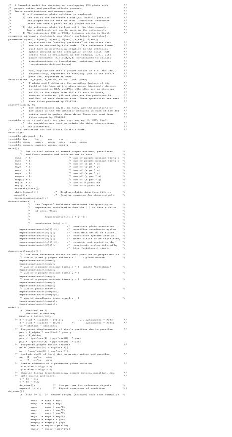
The model file, required by gaussfit, specifies the observed quantities, data items, variables, and parameters. The observed quantities might be the (x,y) positions of the stars in the FGS detector coordinate system as measured in a given HST orbit. “Data” could be the time (e.g., the Modified Julian date) of an observation or roll angle of HST. Variables are quantities calculated from the observations, data, and parameters. Parameters are entities whose values are to be solved for, subject to constraints, to find the minimum on the Chi-Square manifold, i.e., the best global solution that combines the multi-epoch data. For a simple parallax program the “observations” are the (x,y) positions of the science target and reference stars measured in each of the proposal’s HST orbits. The “data” are the star IDs, their (approximate) celestial coordinates, and the HST roll angle and time at each epoch. The parameters are the parallax and proper motion of each star relative to the field. The rotation, translation, and scale changes of the FGS detector space coordinate system from an HST visit relative to a chosen fiducial are determined by additional parameters (invoking the 4 or 6 parameter plate solution). The variables are the quantities that relate the data and observations to the parameters. The model defines the relations between the parameters that form the constraints that the solution must satisfy.

The “observations” and “data” are read in from the output *.tab files generated by the pipeline component CALFGSB. The parameters are specified in the model file. Their initial input and final output values are recorded in the “parameter files” associated with the data reduction process (as discussed below).

The syntax and structure of the model emulates a pseudo C program, and is best demonstrated by the following example. The text below displays the contents of a gaussfit model file that is appropriate for determining the parallax and proper motion of star “1” relative to field stars. In this example the reference field stars (stars != 1), are constrained to have no bulk parallax and proper motion, i.e., the sum of all reference star proper motions is constrained to zero. Some of the reference stars might have a detectable parallax or proper motion relative to the most distant stars in the field. gaussfit will compute a “positive” parallax for these and a “negative” parallax for the more distant stars (since the sum is constrained to zero). It might be appropriate to iterate the process whereby stars with detectable motions are excluded from the constrained sums, and their parallax and proper motions are solved for as part of the grand solution. The “template” shown here is available for download from the FGS Website.

It is worth noting that the parallax and proper motions computed by gaussfit are, of course, relative to the reference stars that were also measured by the FGS. To determine an object’s absolute parallax, one must apply the relative-to-absolute correction. This is typically done by identifying each star’s spectroscopic type and luminosity class, and then from the HR diagram, determining its distance. From this an average distance, and hence parallax, for the reference field is computed. This parallax adds to the science target’s relative parallax, yielding the target’s absolute parallax. More sophisticated applications of gaussfit include the spectroscopic distances as “observations” which are constrained by the uncertainties in the spectroscopic analysis. If feasible, this enhances the reliability of relative-to-absolute parallax correction.

Preparing the Output Products of CALFGSB for Gaussfit

CALFGSB applies a variety of corrections to the (x,y) centroids of the observed stars. The final corrections applied by CALFGSB are for drift of the HST focal plane over the course of the orbit during which the stars’ relative positions were measured. CALFGSB applies two standard models to remove HST/FGS drift: a 2^nd order translation model, and a first-order translation plus rotation model. The Chi-Square fits of the data to each of these models is computed and recorded in the *log file. In a standard CALFGSB execution, the centroids for the 2^nd order translation model are grouped into two columns in the *_ast file (named Xvaofadapj2d and Yvaofadapj2d), while the centroids from the first-order translation plus rotation model are grouped into two additional columns (named Xvaofadapjrd and Yvaofadapjrd). However, the gaussfit model displayed above requires as input the “observation” values (X,Y). The CALFGSB output product (*_ast) should be edited to modify either the pair of column names:

or

The choice of which pair to specify as the “observation” (X,Y) should be based upon whichever drift model yielded the smallest Chi-Square residual (from inspection of CALFGSB’s *.log file). Incidentally, the name Xvaofadapj2d derives from the fact that the X-position centroid has been corrected for - in sequence - differential velocity aberration (va), optical field angle distortions (OFAD), asphere and pickoff mirror distortions (ap), spacecraft jitter (j), and finally the HST/FGS drift (2d or rd models). The reason why (Xvaofadapj2d, Yvaofadapj2d) are not specified as the “observation” in the gaussfit model is because it is generally necessary to combine data from many epochs of HST observing to determine the scientific objective. It may be best to extract the centroids corrected with the second-order translation model for some of the epochs and those corrected with the first-order translation plus rotation model in the others. Editing the data files to specify (X,Y) provides the flexibility to enforce this choice.

The parameter files

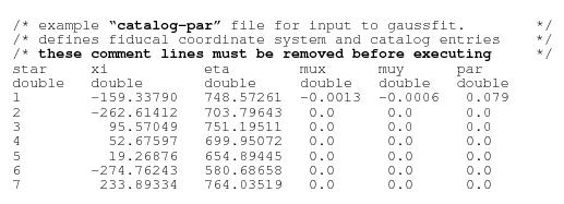
A gaussfit parameter file contains data gathered into columns and rows. Each column is labeled with the name of a particular parameter, as it appears in the gaussfit model file. Each row contains the values of all the parameters for the particular entity defined by the row, such as a star. The example shown below displays the contents of the file “catalog-par” that would be needed to run gaussfit with the model file presented above. The file provides for an initial estimate of each star’s position (xi,eta), proper motion (mux,muy), and parallax (par).

Note that for each star in the FGS observations, there must be an entry in the “catalog-par” file containing an initial estimate of the star’s “catalog position” in (xi,eta) space (see below), the star’s proper motion (mux,muy, in arc-seconds/day), and parallax, (par, in arc-seconds). In the example model shown above, these correspond to the model statement;

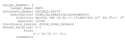
The “star” number in the catalog-par file is nominally derived from the corresponding value of “Target_Number” in the RPS2 phase2 proposal. For example, star = 5 would be assigned to an observation of a star defined in a proposal’s RPS2 target list as:

Note that astrometry programs typically span several HST observing cycles, and therefore may have several phase2 proposals associated with the investigation. This may result in situations whereby a given object is assigned different values of “Target_Number”, and hence “star” across proposal boundaries. In such instances, one must manually edit the CALFGSB output products so that a unique value of “Star” is assigned to each object for all epochs.

In the current example, the gaussfit model also contains the statement:

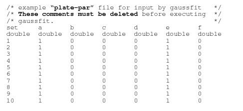
These parameters define the transformation (translation, rotation, and scale) of the coordinate system (the FGS X,Y frame) specific to one epoch on to that constraint epoch, or plate (as can be seen from the model file). This accommodates the fact that the observations across epoch boundaries are generally made at a variety of different spacecraft roll angles and attitudes. In the current example, the initial values of these transformation parameters are contained in the file “plate-par”, whose content is displayed below. Note that there will be one row for each orbit of HST FGS astrometry data in the observing program. Thus in this example, the astrometry program spans 10 orbits of HST observing. The value assigned to “set” is determined by user input to CALFGSB. It is most convenient (but not required) that the data obtained from the program’s first HST orbit are assigned to set=1, and all others are automatically assigned to (set+i), where i sequentially increments by one for each additional entry in the “day.list” file associated with the execution of CALFGSB. (Note that the ordering of the data sets in the day.list file need not be sequential in a temporal sense, although such ordering is highly recommended to minimize confusion when analyzing the results fully reduced data sets.)

While the first parameter file contains data relating to the astrometry of each star, the parameters in “plate-par” contain the values needed to transform the FGS (x,y) coordinate system from each HST orbit (or set) on to the (xi,eta) fiducial coordinate system displayed in the “catalog-par” file. Finally, the fiducial coordinate system is determined from the set which is constrained in the model. In the example gaussfit model file displayed above, this is set = 1, enforced by the statements:
In this case (xi,eta) will be the same coordinate system as (x,y) from observation set 1.Note that to align this to the celestial sphere, (x is east, y is north) one must rotate the coordinate system (clockwise) by an angle computed from the HST V3roll angle of set 1. For astrometry with FGS1r, this is angle given by (V3roll - 90).

Preparing the Catalog Parameter File

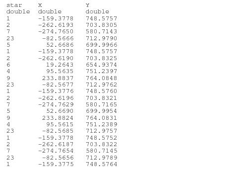
The initial “catalog-par” file can be conveniently constructed by editing the output product from CALFGSB (the *_ast file) of the data set which will also define the fiducial (xi,eta) coordinate system. Once the *_ast file has been edited so that either (Xvaofadapj2d, Yvaofadapj2d) or (Xvaofadapjrd, Yvaofadapjrd) becomes (X,Y), the columns (star, X, Y) should be extracted and written to the “catalog-par” file. This can be done using the utility “extract”, a tool composed of C modules which can be downloaded from the FGS Website. The Makefile needed to generate the executable is included in the tar file.

Once the executable has been generated, one types “extract” (or its alias) while in the local directory containing the *_ast file to be input.extract prompts for the name of the input file to be read and the output file to be created (assumed to be “catalog-par” for this discussion.) extract displays the name and number of each column in the input file and prompts for the column numbers to be extracted; one should enter the numbers of the columns named (Star, X, Y). This will generate an output file with the following characteristics:

Note that there will generally be multiple entries (rows) for a given star since stars are usually observed several times over the course of an HST orbit. The output file should be edited to remove all multiple entries to leave only one row for each star. Generally, it does not matter which rows are retained and which are deleted; at this time the significance of a row in this file is to denote a catalog entry. The actual coordinates that appear will be over written by gaussfit when the final catalog is generated.

In keeping with the example gaussfit model, additional edits to the “catalog-par” file are needed. The columns named (X,Y) should be renamed (xi,eta). Three additional columns need to be created. These are (mux, muy, par), for proper motion and parallax. The second row, which specifies the data type of the column (“double”, for "double precision variable" in this example), needs to be added for each new column. The values entered in each new row can either be zero or an initial estimate of the appropriate entity’s value. Note that proper motion has the units arc-seconds/day, and parallax has the units arc-seconds.

Preparing the Transformation Parameter File

In the example gaussfit model presented on the preceding pages, a parameter file is also required to accommodate those parameters which define the translation of a given set’s (X,Y) coordinates on to the fiducial (xi,eta). The current example employs a 6 parameter solution to make this coordinate transformation. The “plate-par” file will satisfy this need. Note there are 6 columns (a,b,c,d,e,f) and one row for each data set. A template of this file can be downloaded from the FGS Website. The template should be edited to either add or delete rows as needed to match the number of data sets available for the analysis on hand.

Preparing the Environment File

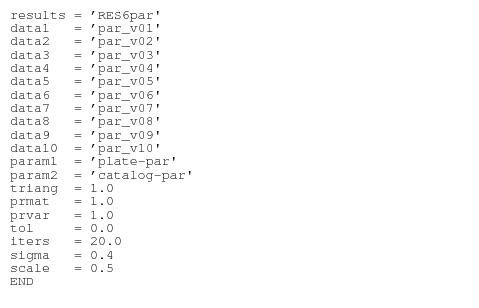
gaussfit inputs an “environment” file from the command line. The environment file specifies the names of the data sets to be input, which are in fact the *_ast files created by CALFGSB (renamed in this example to par_v01, par_v02, ... , par_v10, where v01, v02, etc. correspond to visits 01, 02, ... , 10 for a parallax program with data from 10 HST visits). The environment file also identifies by name the catalog parameter file and the transformation parameter file (“catalog-par” and “plate-par” in this example). The entry RES6 specifies the root name of various files that will be created and written to by gaussfit to record intermediate results from each iteration in the convergence process. These are not particularly useful for non-developers (of gaussfit) and will not be discussed further.

Note that there must be a row in the “plate-par” file for each data set identified in the environment file. For example, the environment file shown below identifies 10 data sets (par_v01 through par_v10). Therefore, the “plate-par” file must identify 10 data sets as well. Shown below is the contents of environment file (named envfile) appropriate for the gaussfit example under discussion.

Running gaussfit

With the model, environment (envfile), and parameter files (“catalog-par” and “plate-par”) properly prepared, and the appropriate output products from CALFGSB (the *_ast files or renamed versions of them specified in the envfile) edited to rename a pair of columns X and Y, one is finally ready to execute the gaussfit program. This is done from the command line, simply by typing:

where “model” is the name of the model file and “envfile” is the name of the environment file. gaussfit reads the environment file to identify the input data files and parameter files, which are then read in. gaussfit reads the model file for instructions on how to relate the observations to the parameters subject to the constraints stated in the model. A least squares approach is iteratively utilized to find the solution with the global minima on the Chi-Square manifold. The results of this process are written into the parameter files. The initial (input) values of the parameters are overwritten with the values determined from the solution, New columns with the “deltas” and “sigmas” for each parameter are added to the parameter files. The data files (par_V01, e.g.,) have columns _X and _Y appended to them. Their row entries record the “error” of the X,Y measurement of the star’s position for each individual observation relative to the derived catalog position (in the coordinate system of the visit).

For the model under discussion in this example, the most interesting quantities to result from this analysis are the new values for the proper motion and parallax (mux, muy, par) and their errors (sigma_mux, sigma_muy, sigma_par). Also of great interest are the residuals of the catalog positions (ξ,η), namely (sigma_xi, sigma_eta). In the example presented here, these residuals are recorded in the file “catalog-par” revised by gaussfit.

A note of extreme caution. gaussfit overwrites the input parameter and data files. If it is necessary to rerun gaussfit on the same data after one or more outlier observations have been removed, it may be desirable to restore the parameter files to their initial condition. For this reason it is best to maintain a “/backup” directory which contains the initial parameter and data files. If single observations are to be removed from the analysis, the data files (par_V01, e.g.) can be edited to delete the troublesome data. If data from the entire visit are to be ignored in the analysis, the environment file “envfile” and the “plate-par” file will need to be appropriately edited to remove pointers to the undesirable visit. Finally, if a given reference star is to be deleted from the analysis for all visits, it needs to be removed from all of the data files and the “catalog-par”. (Actually the model file can be modified to ignore the specific star, e.g. “if (star != 1)”.)

Displaying the Residuals; plot-rss

STScI has developed a convenient tool that can be used to display the residuals of an astrometric catalog generated using gaussfit on the output from CALFGSB. This tool, plot-rss, can be downloaded from the FGS Website. It is composed of C and Fortran modules that call SMSM for plotting. (You may need a site license for SM. STScI is working to replace the SM component with a publicly licensed graphics package.)

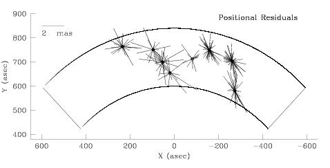
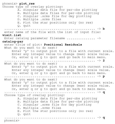
On the following page, a terminal session where plot-rss was invoked to plot the astrometric residuals of the individual measurements of star positions relative to their catalog positions derived (from these individual observations) using gaussfit. User input is in bold. Figure 4.3 shows the plot generated by plot-rss in this example.

Note from the dialog in the terminal session that a variety of results can be displayed. In this particular case, the file “visit.list”, generated by the simple unix command “ls par_V* > visit.list”, contains the names of the data files that have been processed by gaussfit (par_v01, par_V02, etc., for example). plot-rss also prompts for the name of the catalog parameter file (catalog-par), which defines the location of the stars in (xi,eta) space, and is used to plot their catalog positions in the FGS. plot-rss reads the data files and extracts (star, _X, _Y), where “star” identifies the catalog entry (and provides a map to its catalog position). _X and _Y are the residuals of the star’s measured position for that particular observation (relative to its catalog position). plot-rss plots the vector (_X, _Y) with its origin located at the catalog position of “star”. The scale length of the vector can be adjusted as needed to optimize the usefulness of the display. In the case of Figure 4.3, the scale length of 2 mas, as indicated on the plot, was chosen.