4.4 Transfer Mode Data Analysis
Transfer Mode observations with the FGS can resolve the individual components of multiple star systems and measure the angular diameters of extended objects. These observations scan the FGS’s instantaneous field of view (IFOV) across an object to accumulate the necessary data for a post observation reconstruction of the x and y axis interferograms, or S-curves. By comparing the observed S-curves with those from a single (point source) reference star in the calibration database one can deconvolve the contribution of each component in a multi-star system or each chord of an extended object. Such an analysis can reveal the magnitude difference and relative separation and position angle of a binary star system or the apparent angular diameter of an extended object in both the x and y directions.
Routine pipeline processing of Transfer Mode data by CALFGSA, (discussed in Chapter 3), is confined to locating the individual scans within the data files, editing out bad data, and computing guide star centroids and standard deviations during each scan. The CALFGSA output consists of a variety of files to be used by the analysis packages discussed in this section.
Although some observers have used the FGS in Transfer Mode as a photometer or to measure the angular diameters of giant stars, by far the most common use of Transfer Mode has been to resolve close binary or triple star systems to measure the component separation(s), position angle(s), and relative brightness(es). A multi-epoch program that monitors a binary over time can derive its visual orbit. Unlike radial velocity studies, an orbit determined by the FGS reveals the system’s inclination. Additional information about the system’s parallax (which can be obtained by FGS Position mode observations) or radial velocities (for double lined spectroscopic binaries) can be used to determine the component masses.
To provide some background for the analysis of Transfer Mode observations, we briefly discuss the interferometric response of the FGS to the wavefront from a point source and a binary star (for a detailed discussion, please consult the FGS Instrument Handbook).
Single Stars (Point Sources)
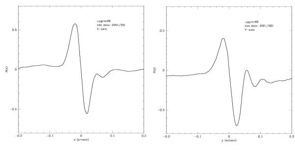
The wavefront of a point source at the face of a Koester prism (the interferometric element of the FGS optical train) is collimated, coherent, polarized, and characterized by a propagation vector. As the instantaneous field of view of the FGS scans across the target, the tilt of the wavefront varies and the PMTs register different relative intensities. Plotting the position of the IFOV along the scan path against the normalized difference of the PMTs reveals, for example, the characteristic point source X and Y axis interferograms, or S-curves, of the FGS1r (Figure 4.4). Note that the response along the X-axis is different than that along the Y-axis. This is due to a slight difference in the alignment of the FGS optical axis along X and Y relative to HST’s OTA. These misalignments, coupled with HST’s spherical aberration, produce higher order aberrations which effect the X and Y axis interferograms differently. (The X-axis S-curve is nearly ideal.) These small aberrations do not degrade the instrument’s performance; performance tends to be limited by the S-curves’ temporal stability and spacecraft jitter, factors that become more important as one attempts to resolve structure on smaller scale (nominally below ~15 mas).
Binary Stars
If the source is a double star, then its wavefront will have two components, each coherent with itself but incoherent with respect to the other. Two propagation vectors characterize this wavefront and the angle between them is directly related to the angular separation of the stars on the sky. As the FGS’s IFOV scans across the object, each component of the wavefront generates its own (point source) S-curve, whose amplitude is reduced by the non-coherent “background” contributed by the other star.
If the angular separation of the stars is greater than the characteristic width of an S-curve (about 60 mas), two distinct S-curves will be apparent, but the modulation of each will be diminished relative to that of a single star by an amount depending on the relative intensity of the stars.
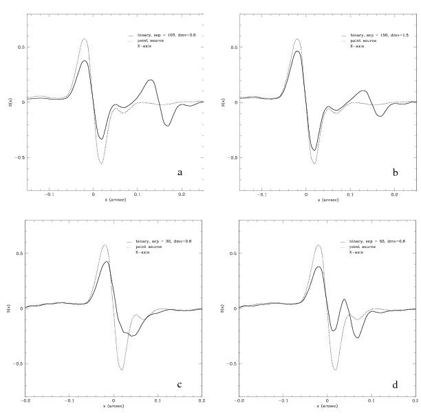
For illustration, Figure 4.5 shows X-axis interferograms to be expected from (a) a binary with a separation of 150 mas and δmv = 0.6 and (b) the same separation as (a) but with δmv=1.5. For reference the S-curve of a point source (dotted line) is superimposed on that of the brighter component in both (a) and (b).
On the other hand, if the angular separation is sufficiently small, the S-curves will be superimposed, and the morphology of the resulting blend will be complicated. Figure 4.5 shows the X-axis S-curves to be expected from a binary system with a δmv = 0.6 and (c) a separation of 50 mas and (d) a separation of 30 mas. As in Figure 4.7 a and b, a point source S-curve (dotted line) is superimposed on the brighter component in (c) and (d) for reference.
In either case, the composite S-curve can be deconvolved using reference S-curves from point sources, provided the angular separations are not too small and the magnitude difference is not too large. To be more precise, fitting the observed double star S-curve with two appropriately weighted, linearly superimposed reference S-curves from single stars can determine the projected angular separation and magnitude difference of the binary’s components along each FGS axis. By combining the X and Y data the binary’s true projected angular separation and position angle can be measured.
Transfer Mode and Faint Targets
The modulation, morphology, and temporal stability the point-source S-curves ultimately determine the resolving power of an FGS for objects brighter than V ~15. For fainter objects, the photon noise inherent in the individual scans makes cross correlation of the individual scans more challenging, which in turn makes the removal of spacecraft jitter more difficult. FGS1r has successfully observed stars in Transfer Mode as faint as V=16.6 with good S/N. However the loss of fringe visibility, due to the dark + background light, which is comparable to the source for such faint targets, probably degrades FGS1r’s angular resolution to about 12 mas (compared to ~7 mas for brighter stars) for binaries with δmv< 2.
4.4.1 Transfer Mode Data Reduction
The astrometry pipeline routine CALFGSA locates and extracts the individual scans of a Transfer Mode observation. As discussed in the previous chapter, files with names such as rootname.1s1, rootname.1s2, ... , rootname.isj, are output, where rootname identifies the observations (i.e., f4mb0602m), i = fgs_id (1,2,3) and j = scan_id. Files for all three FGSs are output by CALFGSA (unless one of the guiding FGSs is inactive, i.e., not tracking a guide star, in which case no files for that FGS are output).
The analysis package “ptrans”, available for download from the FGS Website (http://www.stsci.edu/instruments/fgs/), is a convenient tool for the processing CALFGSA output files. ptrans takes as input the rootname.isj files for the astrometric FGS and cross correlates, co-adds, and smooths the co-added S-curves in an interactive, iterative fashion. During the process, individual Transfer Mode scans can be plotted against the current iteration’s co-added S-curve. Data from individual scans can be evaluated for quality and corruption (from space craft jitter). Individual scans can be eliminated from the next iteration’s co-addition process (if desired). As with the other FGS analysis tools that offer graphical output, the current package utilizes SM. A site license may be needed if you wish to port ptrans to non-STScI sites.
Aside from the graphical displays and data quality assessments, ptrans performs the following routine operations on the input scan data:
- Cross-correlation of each scan in order to detect any drift of the FGS across the sky during the course of the observation. Cross-correlation is an option that can be declined. This might be appropriate when processing observations of objects fainter than V~15 since the data from individual scans are photon noise dominated to such an extent that cross correlation becomes increasingly unreliable (i.e. harmful) with increasing V magnitude.
- Shifting of each scan by the amount determined necessary in step (1) so that all scans are mapped to a common reference frame. If the option to cross-correlate is declined, no shifts are performed.
- Co-adding the individual scans to generate a high signal to noise ratio (S/N) S-curve. Each step of the IFOV along each scan is placed into an appropriate bin, and then all entries in a given bin are averaged to produce the high S/N co-added S-curve.
- Fitting of a piece-wise third-order polynomial fit to the binned and co-added S-curve. ptrans provides the user with the ability to interactively fine tune the smoothing process. This helps to avoid imposing false artifacts into the final product on the one hand but also yields the highest (reliable) S/N final product.
If the observation under analysis is of a binary star system and the observer wishes to determine the angular separation, position angle, and magnitude difference of its components, the following additional steps are undertaken. - Select the appropriate set of reference S-curves from the calibration library on the basis of the target color (or colors) and the dates of observation of both the binary system and the calibration stars. These dates should be as close as possible to minimize the impact of temporal variations in the particular FGS. (FGS3 was the astrometer before cycle 8, FGS1r has been the astrometer since.) The appropriate calibration data files can be downloaded from the FGS Website; follow the links to calibration data files.
- Use the tool “binary-fit”, also available for download from the FGS Website, to determine the component angular separation, position angle, and magnitude difference. This fitting is done on both the x and y axis. binary-fit inputs the products from ptrans, the rootname.tab file from CALFGSA, and the appropriate files gather from the STScI FGS calibration library in step (4).
The following sections describe the tools ptrans and binary-fit. Detailed instructions in their use, supported by examples captured from terminal sessions, are provided.
ptrans
The analysis package ptrans is composed of Fortran and C source code. ptrans inputs the rootname.isj products output by CALFGSA for Transfer Mode observations. ptrans makes extensive use of graphical output (calls to SM graphical routines). ptrans is available for download from the FGS Website. The source code and necessary Makefiles and README files are available in the tar ball.
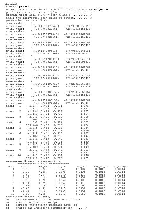
Once an executable image of ptrans is available, one prepares for using the package by gathering all of the observation’s rootname.isj files into one directory. Then, while in that directory, simply type ptrans.e or its alias to activate the tool. Displayed below is the first iteration of ptrans captured from a terminal session while processing a Transfer Mode observation of a calibration point source. This particular observation of a bright source (V=9) had only 10 scans. User input is in bold.
The user is next offered the choice to have ptrans perform cross correlation of the individual scans so they can be shifted (to eliminate space craft jitter and/or drift). Simply entering <ret> defaults to invoke cross correlation. The option to decline may be appropriate for faint objects (V > 15) whose individual scans are dominated by photon noise rather than spacecraft jitter/drift. In such cases it is recommended that the analysis be tried both with and without cross correlation and the output be compared.
The next option - to process the scan data along only the x or y axis, or both - occurs if one simply enters <ret>. This option is convenient in situations where there is known to be useful data along only one of the FGS axis (a determination that can be quickly made using fgsplot), or in situations when a smoothed and co-added final S-curve of satisfactory quality is already available for one of the axis (and there is no need or desire to repeat the processing of that data).
Next, ptrans offers the option to output the individual scan files. If this option is invoked, files with names such as rootname.x1, rootname.x2, ... , rootname.xn, will be output. The contents of each will be a listing of (X,Sx) for the given scan, where X is the location of the FGS IFOV along the scan path, and Sx is the instantaneous value of the S-curve along the x-axis for that 40 Hz sample. The same holds true for the rootname.yi files along the y-axis. This capability is usually not invoked. However it can be useful for analysis when confronted with garbled data or instances of high spacecraft jitter.
Once the initial input is provided, ptrans completes the setup by reading in and processing the data in all of the scan files. As discussed in the previous chapter, these files contain the star selector servo rotation angles (from which the IFOV x,y coordinates are computed), and the counts/25msec from the four PMTs. From these data the S-curves of the individual scans are re-constructed. The first set of screen output shows the (x,y) start and stop end points of each scan. This can be useful for quickly verifying the completeness of each scan. The next set of screen output shows data for each scan grouped into two rows. The first row shows the mid point of the x-axis scan and the +/- peaks of the value of that scan’s x-axis S-curve. The second row shows the equivalent data along the y-axis. These data can also be useful for trouble shooting or identifying bad scans. At this point ptrans has completed the initial setup.
The results from the initial iteration are displayed next. Statistical data for each scan are presented in rows. The first column (scan) identifies the scan; the second (shift) displays the amount of shift, in milli-arcseconds (mas), deemed necessary by cross correlation; the third column (rel_diff) is a ratio of the values in columns 4 and 6; while the fourth column (sd_fr) shows the standard deviation of the individual scans’ S-curve relative to this iteration’s co-added (but not smoothed) scan. These values are computed via the relation:
where Sc(i) is this iteration’s co-added S-curve at position x(i), Sj(i) is the value of scan j’s S-curve at position x(i), and the range in i (=m to n) covers only the central 100 mas of the scan, to assure that only the fringes (and not the wings) are included in the calculation. Thus, the values in column 4 provide a rough estimate of the quality of the individual scans. The value in column 6 (ave_sd_fr) is simply the average of all values in column 4. The values in column 3 (rel_diff) is a more user friendly method of identifying the true outliers in column 4. Column 5 (sd_wg) is similar to column 4 (and is computed in the same way), except that the summation integral is restricted to the wings of the scan. This provides an assessment of the photometric noise in the S-curves, which is dominant in the wings (the wings of the S-curves are not sensitive to spacecraft jitter). Finally, column 7 (sd_wings), shows the standard deviation of the co-added S-curve compared to the best fit straight line in the wings of the scan, yielding insight about the photometric noise present in the co-added scan.
At this point the user is prompted to provide input for starting the next iteration. The first choice “enter scan numbers to omit”, allows for specific, individual scans to be eliminated from consideration in the next iteration. These can be identified by scan number(s). If more than one is to be eliminated, the entries should be delineated with either comas or spaces. Note, entering a negative scan id, e.g., -3, will force scan #3 to be included in the next iteration. This can be useful if scans are inadvertently deleted, or to restore the quality of the final co-added S-curve if it is found to degrade when specific scans are deleted.
The second choice, “set maximum allowable threshold (fx.xx)”, allows for the user to eliminate all scans whose value in column #2 (rel_diff) exceeds a specific (entered) value, e.g., f1.15 would disqualify scans 1,4,9 in the example sited above (note the "f" must be entered to allow ptrans to apply this option). Invoking this option can be convenient when processing observations with a large number of scans (typically > 50).
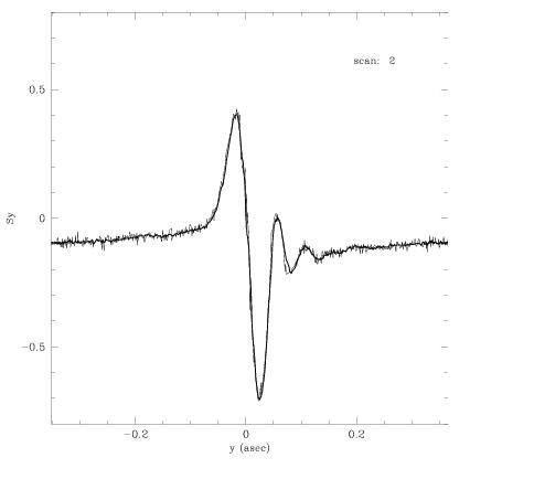
The option to “choose to plot a scan (p#)” offers the ability to explicitly view a particular scan’s S-curve and compare it to the current iteration’s co-added (but not smoothed) S-curve. This can be useful when deciding whether or not to delete or retain scans that appear questionable on the basis of values shown in the 7 columns. If a particular scan is to be plotted, ptrans displays the (min,max) of the scan path (in x or y, depending upon which axis is being processed at the moment). The user is prompted to choose the segment of the scan path to be plotted. Entering “a” plots the entire scan, entering “s” plots the same segment that was chosen for the last plot (if this is the first iteration, entering “s” plots the entire scan). If numerical values for xmin and xmax are entered (instead of <ret>, a, or s), the user is prompted to set the vertical limits of the plot. Entering <ret> sets the vertical limits to +/- 0.8, which is a convenient standard.
Once a plot is generated, the user is offered the opportunity to direct the plot to a postscript file (“output the plot to a file?“). If this option is invoked, a file named scan_jX.ps is generated, where j is the scan_id (and the X-axis is being processed in this example). Subsequent plots of scan j’s X-axis S-curve will over write this file.
The user is next presented with the opportunity to re-plot the data with different limits along the abscissa and ordinate. Entering <ret> defaults to “no”. The user can mark the scan for deletion in the next iteration, and finally can plot a different scan (specified by scan #). The extracted terminal session segment shown below illustrates this interaction.
|
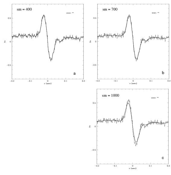
allow for a fine tuning of the parameter “sm” which determines the degree to which the co-added S-curve is smoothed. The smoothing algorithm applies a third-order polynomial approximation to segments of the scan data. The length of the segments determines the degree to which the S-curve is smoothed. The value of sm, in part, determines the length of these segments, and hence the degree to which the scan is smoothed. Too little smoothing (small sm) needlessly retains noise in the final S-curve. To much smoothing (sm too large) suppresses signal, which compromises the scientific conclusions one might make about the observation.
Figure 4.7 shows a comparison of smoothed vs. unsmoothed S-curves for three different values of sm: 400, 700, 1000 (in panels a, b, and c respectively). These data are from an observation of a V=15.6 white dwarf star. The photometric noise in the wings of the fringe is apparent in the unsmoothed data. A value of sm=400, does a poor job of suppressing the noise, as is evident in the how closely the smoothed curve tracks the noise in the wings. On the other hand, a value of sm=1000 over suppresses the noise and results in the poor fit of the smoothed data within the S-curve peaks. The optimal value, sm=700, smooths out the wings while retaining a good fit to the S-curve.
The last option, “change the smoothing parameter (sm)”, displays the smoothed, co-added S-curve without the unsmoothed, co-added S-curve superimposed. As with the other options, the display can be output to a PostScript file if desired.
ptrans output
In addition to plots of Transfer Mode observations, ptrans generates three ASCII files listing x and S(x) of the co-added S-curve. These files follow the nomenclature
|
where rootname identifies the observations (e.g., f2bm0203m);
Similar files are generated for the y-axis data (*.cy, *.cy0, *.cy0s). The “shift” refers to a redefining of the x-axis coordinate system such that x=0 corresponds to the so-called zero point crossing of the S-curve, which is between the positive and negative peaks of the fringe. The plots displayed in figure 7 were all generated from the *.cxo and *.cx0s files. This zero point is also referred to as interferometric null, or the null point crossing. The same applies to the y-axis S-curves.
Two other files of interest - "xy.shifts" and "rootname.zero_point" - are ptrans products. “xy.shifts”, which records the shift of each scan as a result of the cross correlation procedure. If the option to cross correlate was declined, the shifts will be 0. The final file, “rootname.zero_point”, lists the actual (x,y) location of the S-curve zero point crossing in FGS detector space coordinates (the same coordinate system used in the *.cx and *.cy files). It also lists the amplitude of the +/- peaks of the S-curves for both the x and y-axis.
Files “rootname.cx0s” and “rootname.cy0s” are the main products of ptrans. Each contains the data-quality edited, cross correlated, co-added, and smoothed interferometric fringes of the observed target. This is the fully optimized S/N product of the observation. If the object is a binary system, for example, it is these files that serve as input to the binary star analysis package to be discussed in the next section. On the other hand, if the observation is of a point source calibration star, these files will become part of the FGS calibration library, and will serve as the point source “templates” needed for the analysis of Transfer Mode observations of binary or multiple star systems.
4.4.2 Analyzing Observations of Binary Stars
The most common use of the FGS as a science instrument in Transfer Mode is to resolve binary or multiple star systems. Because it is possible to sample the FGS’s interferometric fringes in steps of ~1 mas, binary systems with separations well below HST’s diffraction limit (down to ~10 mas) can be “resolved” by applying a model which compares the observed fringes of the target system to those from a (unresolved) point source. The point source calibration fringes are available from the FGS calibration library, and files containing these data can be downloaded from the FGS Website.
Members of the Space Telescope Astrometry Team (STAT) from Lowell Observatory developed an analysis package which can be used to deconvolve the composite fringes of a binary star system to yield the separation, position angle, and relative brightness of the binary’s components. The package employs a four-dimensional least squares algorithm to find the best fit (minimum Chi-square) of superimposed point source fringes to the observed binary star fringes. The four “dimensions” here refer to star separation projected along an FGS axis, the relative brightness of the components, the location within the scan of the brighter component, and a bias term which accounts for changes in the sensitivity of the photomultiplier tubes over the time between when the science data and calibration data were obtained.
This package has been made available to STScI, and has been modified by the STScI FGS group to account for the effect of (dark + background) photon counts in order to accommodate the analysis of faint (V > 14) binary systems. To facilitate an evaluation of the quality of the model fit to the observed data, STScI has further enhanced the package to graphically display an overlay of the observed binary star interferogram with that of a “synthetic binary” generated from the point source calibration data (using the derived values for star separation and relative brightness).
This Unix/Linux based analysis package, referred to as binary-fit, is composed of Fortran and C modules. The source code and associated Makefiles can be ported by download from the FGS Website.
binary-fit
Once an executable image of binary-fit is built on the host machine (using the source code and Makefiles provided by STScI), and an alias pointing to the executable is specified, the tool can be run by simply typing binary-fit (or some other user defined alias) while residing in the directory containing the files needed for input.
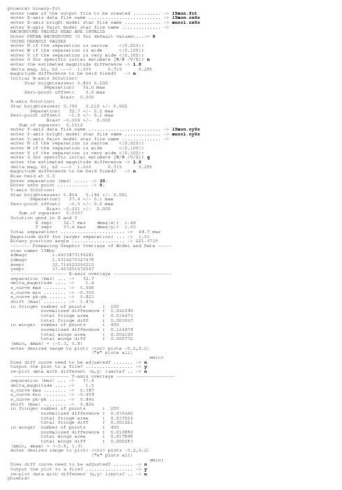
binary-fit takes as input the *.cx0s and *.cy0s files generated by ptrans. These files, containing the co-added and smoothed interferograms, are needed for both the science target and the point source calibration star (which can be obtained from the FGS Website). Also needed are the *.tab files (generated by calfgsa) associated with both the science and calibration observations. Initially, binary-fit determines the projected component separation and magnitude difference (δmv) along the FGS x and y axis independently. However, the δmv of the stars should be the same along both FGS axis. binary-fit enforces this constraint (to within a small tolerance). If there is significant disagreement between the results along x and y, the user is prompted to identify which axis is to be refit (for component separation), with the constraint that the stars’ δmv is held fixed at the value determined along the other FGS axis. The choice of which axis to refit is usually based upon the quality of the fits along each axis (the Chi-Square values), i.e., refit the axis with the highest Chi-Square, or by adopting the δmv determined from the axis with the wider projected separation of the stars. Examples of this are presented below.
An estimate of the relative brightness and separation (along an FGS axis) of the binary’s components is useful for defining the region of parameter space that is probed for a minimum Chi-Square solution. These estimates need not be very accurate (especially for relative brightness); they serve only to avoid having binary-fit converge on a local minimum rather than the true global minimum on the Chi-Square manifold. Examples of this are also presented below.
In the following two sections, examples are given for the analysis of “wide” and “narrow” binary star systems. Generally, wide systems refer to cases where the projected separation of the stars is larger than ~70 mas, resulting in two distinct S-curves, as displayed in Figure 4.5a and Figure 4.5b. Narrow systems have smaller separations, resulting in blended S-curves, as seen in Figure 4.5c and Figure 4.5d. Note however that the orientation of HST can be such that the binary’s position angle is nearly aligned with one of the FGS axes. This will result in small projected separation of the binary’s components along the orthogonal FGS axis, so even a wide binary might need to be treated as a “close” binary when analyzing the data along that axis.
binary-fit and wide binary systems
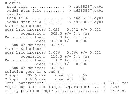
The example shown below displays a terminal session using binary-fit to determine the separation and position angle from observations of the wide binary system SAO85257 (V = 9.5, B-V = 1.2) from HST proposal 8835. The point source calibration star used in this analysis is the V = 9.7 FGS standard HD233877, chosen on the basis of its B-V = 1.1 color which is sufficiently close to that of the binary system (see “Uncertainties in Transfer Mode Data” for a discussion about the effect of spectral color on FGS S-curve amplitude and morphology).
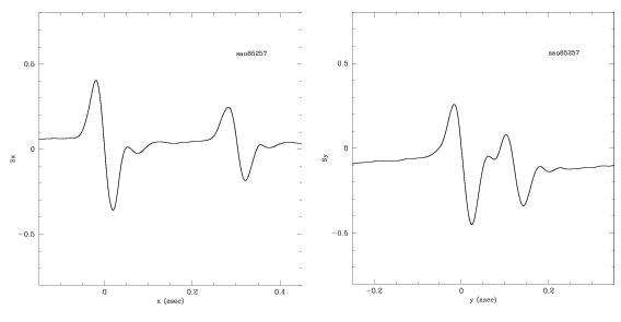
After processing the observation’s raw GEIS files through the pipeline processor calfgsa, the resulting products are processed through ptrans. The graphical output from ptrans, shown in Figure 4.8, clearly shows this to be a wide (sep > 100 mas) binary system a projected along both FGS1r axes. In cases such as this it is easy to estimate the separation of the stars along each FGS axis as well as their magnitude difference, δmv (the relative amplitudes of the S-curves corresponds to the relative brightness of the two stars). These values can be used as initial estimates for binary-fit.
|
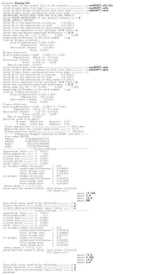
With these files present in the default (current) directory, a session with binary-fit would appear as shown below. The entries in bold are input by the user in response to prompts (“>”) from binary-fit. <ret> is entered for prompts with no explicit response.
BACKGROUND VALUES READ FROM TAB FILE ARE INVALIDEnter PMTXA BACKGROUND (0 for default values)...-> 0USING DEFAULT VALUES
is likewise deferred to the section that addresses the analysis of faint (V > 14) binary stars. (For brighter stars, the default background values are recommended, i.e., respond with a “0”).
The user has the option of entering then name of a “faint calibration star file name”. Because the amplitude and morphology of point source S-curves is a mild function of the spectral color of the source (see “Uncertainties in Transfer Mode Data”), this option is useful in situations where the components of the binary are known to be of different spectral colors (e.g., a B star and a red giant). Note that the star that is expected to be the brighter component (in V) will be represented by the "bright calibration star" reference file, while the fainter component is represented by the “faint calibration star” (where "faint" is used as a relative term in this case). If both components have approximately the same color (δ(B-V) < ~0.2), then only one reference file is needed. By responding to the second prompt with a <ret>, the same reference S-curve will be used for both components in the fitting process.
After solving for (sep,δmv), binary-fit compares the values of brightness ratios computed along both the x and y axis. If they differ by more than 20% the user will be alerted and prompted to specify which axis is to be re-fit. The brightness ratio on that axis will be held fixed at the value computed from the other axis.
Once a solution is achieved along both FGS axes, binary-fit reads the *.tab file associated with the science data to access the HST roll angle at the time of the observation. From this, the binary star’s position angle is computed (the HST roll angle allows for a determination of the orientation of the FGS coordinate system relative to celestial North, while the measured separations δx,δy give the binary’s position angle in the FGS coordinate system).
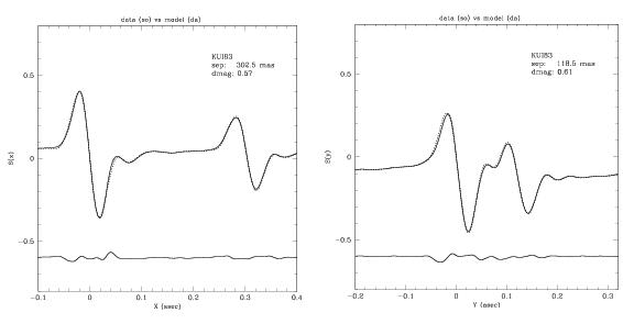
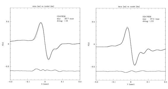
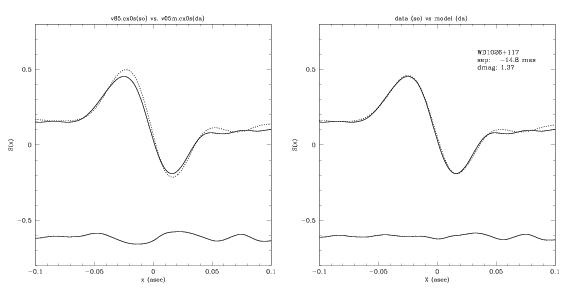
Next, binary-fit generates the fringes of a model “binary star” using the point source calibration data (from the files specified as the bright and faint model stars) and the (sep,δmv) determined from the fitting process. This model fringe is cross correlated and differenced with the science data. A plot showing the overlay of the model with the data, along with their difference, is displayed to screen (see Figure 4.9). These plots can be adjusted for range along the abscissa and ordinate. The difference curve is displaced from 0 (for illustration purposes) by a default of -0.6 units. The user has the option to modify this placement if desired (e.g., if the default displacement causes the difference curve to become superimposed on the data/model curves). Finally, the plot shown on the screen can be captured to a postscript file.
binary-fit output files
Three files are output by binary-fit: the two postscript files containing the data/model overlay, and file TARGET_NAME.fit, where TARGET_NAME is the value specified by that keyword in the science observation’s *.tab file. In the example cited above, TARGET_NAME = SAO85257. Therefore, a file named SAO85257.fit will be one of the output files. The postscript output with the model/data plots will be named SAO85257xfit.ps and SAO85257yfit.ps. The contents of the *.fit file records names of the data and calibrations input files and the details of the derived solution. The *.fit file generated by the example discussed above has the following contents:
binary-fit and close binary systems
The FGS is well suited for resolving binary systems with component separations on the order of and below the HST diffraction limit. In such cases, “resolution” of a binary system results in a composite fringe that is clearly different from that of a point source, i.e., “resolution” does not mean that the observation produces two distinct S-curves. The morphology and amplitude of the composite fringe is a direct function of the projected angular separation of the stars and their relative brightness.
The analysis of a close binary system is carried out in the same way as for wide systems. However, for separations less than ~20 mas, binary-fit may find several different solutions with nearly the same Chi-Square values. In these situations, one solution tends to have a (comparatively) large δmv and large separation, while another solution has a smaller δmv and smaller separation. This underscores the utility of being able to specify and hold fixed the magnitude difference while executing binary-fit, if the δmv is known from another source, such as spectroscopy, or from another FGS measurement (e.g., the binary is observed at a different epoch with a wider separation, or has a wide separation on the other FGS axis in the same observation).
In the example shown below, binary-fit is used to determine the magnitude difference, separation, and position angle of the two stars comprising the O-star binary system 15 Monoceros in NGC 2264. These data show that at the epoch of this observation (HST proposal 7484, PI Gies), the stars had an angular separation of ~35 mas along both FGS axis. The user inputs are shown in bold.
Analyzing Faint Binary Systems
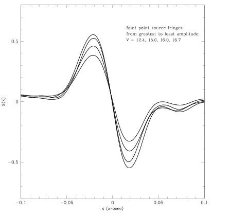
For stars fainter than about V = 14.5, the dark + background counts registered by the FGS photomultiplier tubes (PMTs) becomes non-trivial compared to the counts registered from the source. At about V = 16.5, the source counts are about the same as the dark + background. Since the light from the star is not coherent with the “light” from the dark + background contribution, there is a loss of fringe “visibility”, or amplitude, that becomes more and more dramatic as the instrument’s faint limiting magnitude (V ~ 17) is approached. Figure 4.11 shows the S-curves obtained from scanning faint white dwarf stars (proposal 9169, PI Nelan). The S-curve with the greatest amplitude is from a V=12.4 star and is shown here to demonstrate the FGS fringes when the dark + background is insignificant. The increasingly lower amplitude S-curves are from white dwarfs with V = 15.0, 16, and 16.7, respectively.
The calibration S-curves that populate the FGS reference library of point source fringes were all obtained from observations of stars typically brighter than about V < 9.5. When using these reference fringes to analyze Transfer Mode observations of faint stars, the reference fringes must be adjusted to account for the effect of the dark + background. In essence, the calibration S-curves must be processed to serve as a suitable proxy for point source fringes at the appropriately faint magnitude. The dark + background counts for both the science and calibration observations are recorded in the *.tab files. Using these values, as well as the photometry data (also included in the *.tab files), binary-fit adjusts the calibration S-curve for the dark + background effect.
