4.5.1 Target Selection Criteria

Other than the brightness restrictions specified in Table 4.6 there are several additional considerations when selecting targets for Transfer mode observations.

• Position in the FOV: The morphology of the fringe varies considerably with position in the FOV, as shown for FGS1r in Figure 2.6. As explained in Chapter 2, this field dependence is the manifestation of small misalignment between the star selector optics and the Koesters prism which is greatly magnified by HST’s spherical aberration. To obtain the highest quality data with the best resolution, all Transfer mode observations should be obtained at the AMA optimized position at the center of the FOV. Under normal circumstances, STScI will provide reference S-Curve calibrations only at the center of the Field of View­.
• Color: The FGS’s interferometric response is moderately sensitive to the spectral color of the target. The FGS calibration library contains interferograms from point-source objects with a variety of (B–V) colors. The GO is encouraged to inspect this library to ascertain whether a suitable reference (δ(B–V) < 0.3) is available for data analysis. If not, the FGS group should be alerted, and efforts will be made to enhance the library. The color calibrations available in the FGS library are listed in Chapter 5. Up-to-date additions can be found on the FGS Web site: http://www.stsci.edu/hst/instrumentation/fgs
• Minimum Scan Length: In order for Transfer mode observations to achieve the highest possible signal-to-noise, the length of the scan should be as short as possible (to allow for more scans in the allotted time). The minimum scan length is determined by the expected angular separation of the components of the binary being observed plus the recommended minimum size (for a point source) of 0.3", or,

Min Scan Length (arcsec) = 0.7 + 2x

where the value x is the largest anticipated angular separation of the binary along either axis.

• Minimum Scan Length: In order for Transfer mode observations to achieve the highest possible signal-to-noise, the length of the scan should be as short as possible (to allow for more scans in the allotted time). The minimum scan length is determined by the expected angular separation of the components of the binary being observed plus the recommended minimum size (for a point source) of 0.3", or,
• Maximum Scan Length: When considering the maximum scan length, three concerns should be addressed:

-Masking by the field stops becomes relevant when the FOV is moved beyond 2 arcsec from the photocenter. False interferometric features become prevalent.

-Beyond 2.5 arcsec from the photocenter, the intensity of the target’s light drops off considerably, resulting in poor signal-to-noise photometry.

-Maximum commandable scan length is 6.7".

• Target Orientation: If the approximate position angle of the non-point source is known, then specifying an orientation for the observation may be advantageous. If possible, (for wide binaries) avoid the situation where the projected angular separation along one of the axes is less than 20 mas. Specific orientations are achieved by rolling the HST to an off-nominal roll attitude or by scheduling an observation at a time when the nominal roll is suitable. It should be noted however that special orientations are considered as special scheduling requirements which affect schedulability.
• Target Field: The Search and CoarseTrack acquisition are vulnerable to acquiring the wrong object if the field is too crowded (with neighbors of comparable brightness within 8 arcseconds of the target). Hence, the problem addressed in Section 4.2.7 for Position mode observations applies equally to Transfer mode observations.

4.5.2 Transfer Mode Filter and Color Effects

Table 4.6 is a summary of the available filters and associated restrictions governing their use.

Table 4.6: FGS1r Transfer Mode Filters to be Calibrated During Cycle 8

The S-Curve morphology and modulation have a wavelength dependence. Experience with FGS3 has shown that the color of the reference star should be within δ(B–V) = 0.1–0.2 of the science target. We endeavor to maintain a library of single reference stars which accommodate the color requirements of the GO proposals in the Cycle. These color standards are usually observed once during the Cycle, while Upgren69 is observed every 6 months to monitor S-curve stability.

4.5.3 Signal-to-Noise

In essence, the “true” signal in a Transfer mode observation of a binary system is the degree to which the observed Transfer Function differs from the S-curve of a point source. The signal-to-noise (S/N) required of an observation will depend upon the object being observed; a wide binary whose stars have a small magnitude difference and separation of 200 mas will be much easier to resolve than a pair with a larger magnitude difference and a separation of only 15 mas.

The “noise” in an observation has contributions from both statistical and systematic sources. Photon noise, uncertainty of the background levels, and spacecraft jitter comprise the statistical component. The temporal variability and spectral response of the S-curves dominate the systematic component (these are monitored and/or calibrated by STScI). Provided that at least 15 scans with a 1 mas step size are available, observations of bright stars (V < 13.0) suffer little from photon noise and uncertain background levels, and show only slight degradations from spacecraft jitter (with high S/N photometry, the segments of the data which are degraded by jitter are easily identified and removed from further consideration).

Maximizing the S/N for observations of fainter objects requires a measurement of the background level (see Chapter 6) and a larger number of scans to suppress the Possonian noise in the photometry of the co-added product. But with lower S/N photometry in a given scan, corruption from spacecraft jitter becomes more difficult to identify and eliminate. Therefore, the quality of Transfer mode observations of targets fainter than V = 14.5 will become increasingly vulnerable to spacecraft jitter, no matter how many scans are executed.

Systematic “noise” cannot be mitigated by adjusting the observation’s parameters (i.e., increasing the number of scans). To help evaluate the reliability of a measurement made in Transfer mode, STScI monitors the temporal stability and spectral response (in B–V) of FGS1r’s interferograms. As discussed elsewhere, the FGS1r S-curves appear to be temporally stable to better than 1%, and the Cycle 10 calibration plan calls for observations of single stars of appropriate B–V to support the data reduction needs of the GOs (this calibration will be maintained in Cycle 29). This should minimize the loss of sensitivity due to systematic effects.

4.5.4 Transfer Mode Exposure Time Calculations

The step_size and number of scans determine the number of photometric measurements available for co-addition at any given location along the scan path. Typically, up to 50 scans with 1mas step_size are possible within a 53 minute observing window, (after accounting for overheads and assuming a scan length ~ 1.2 arcsec per axis). The step size and number of scans that should be specified are in part determined by the target’s magnitude and angular extent and also by the need to allocate time within the visit to any other objectives, such as Position mode observations of reference stars (to derive a parallax for the binary). The total exposure time for a Transfer mode observation (excluding overheads) is:

$$//<![CDATA[ \begin{array}{l}\displaystyle \small{T_\mathrm{exp}=\frac{\rm ScanLength}{\rm StepSize}\times(0.025\ \mathrm{sec} \times N_\mathrm{scans})~,}\end{array} //]]>$$

where T_exp is the total exposure time in seconds, N_scans is the total number of scans, 0.025 is the seconds per step, ScanLength is the length of the scan per axis in arcsec, and StepSize is given in arcsec.

Photon noise is reduced by increasing the number of scans, N_scans, as displayed in Figure 4.4, which demonstrates the benefits of binning and co-adding individual scans. Trade-offs between step size, length, and total duration of an exposure are unavoidable especially when considering visit-level effects such as HST jitter.

Simulations using actual data scaled by target magnitude are needed to relate the Transfer Function signal-to-noise (described in the previous section) to the resolving performance of the instrument. A robust exposure time algorithm is in development. In Table 4.7, we offer some guidelines on the minimum number of scans to use in a visit for various binary parameters. These are derived for a step size = 1.0 mas, so that in a 1 mas bin there would be NSCANS samples per bin. Smaller step sizes facilitate the use of less scans to achieve the same signal-to-noise ratio. (Specificity fewer scans with smaller step sizes can reduce the observational overhead, which can increase the time on target and hence the overall signal-to-noise ratio. However, intermittent vehicle jitter may corrupt the data from some scans to the degree that such data is useless for scientific purposes. These trade off need to be considered when planning the observations).
 

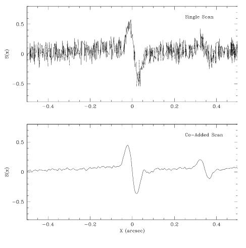
Table 4.7: Suggested Minimum Number of Scans for Separations < 15 mas

¹Note that 60 scans is about the maximum that can be performed in a single HST orbit (assuming a scan length of ~1”). Multi-orbit visits do not necessarily increase the achievable S/N for targets of V >15 since photometric noise makes cross correlation of scans across orbital boundaries questionable. In other words, the data gathered during one orbit is not reliably combined with data from another orbit for faint, close binary systems.