4.5 Displaying Imaging Data
This section will be of interest primarily to observers whose datasets contain two-dimensional images from the imaging detectors onboard HST. We will discuss two methods for displaying imaging data:
- Display of an image using ds9
- Creation of a figure using matplotlib
- Analysis of an image using imexam
4.5.1 Viewing Image Data in DS9
DS9 is a suitable option for displaying data if one simply wishes to view the imaging data contained within a FITS file, or do basic analysis work such as estimating the centroid position of a point source. The ds9 website (http://ds9.si.edu/site/Home.html) contains information on more advanced features including command line arguments. From a bash prompt, one can open ds9 by typing:
ds9 &
This will open ds9 in the background. If the file name is specified, e.g.,
ds9 icdm0a070_drc.fits &
then the image will be displayed. In the case of a MEF file, the first FITS extension (not the zeroth primary extension) will be displayed. To access other extensions, specify them at the command line:
ds9 icdm0a070_drc.fits[2] &
This will display the second extension in the MEF file, which in this case contains weight image of a drizzled observation set. Much of the functionality for adjusting scaling, limits, matching of multiple images using the World Coordinate System (WCS) or aligning in pixel-space can be done using menu options in the ds9 graphical user interface. Some of these features may also be accessed when opening data via the command line. See the ds9 documentation for more information.
4.5.2 Plotting Imaging Data with Python
As discussed in Section 4.4, the data component of a FITS file HDU is read into Python as a numpy ndarray object, and thus it may be treated like any other data array for plotting purposes. We can use matplotlib to visualize the data and create figures.
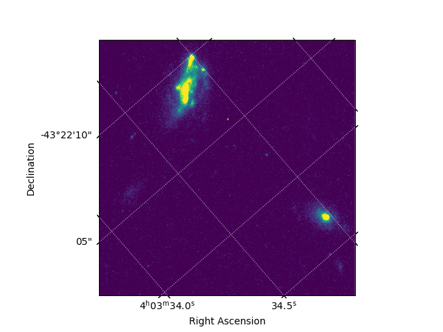
In this example, we will create a plot of a subsection of a WFC3/UVIS drizzled image. We manually set the scaling to display the image, and include right ascension and declination axes. We then save the plot as a PNG image "galaxies_wcs.png".
from astropy.io import fits
from astropy.wcs import WCS
import matplotlib.pyplot as plt

# Open the FITS file and retrieve the data
# and WCS header keyword information from the
# first science extension. Save the WCS
# information into an Astropy WCS object.
with fits.open('icdm0a070_drc.fits') as hdu:
	data = hdu[1].data
	wcs = WCS(hdu[1].header)

# Select a subsection of the image to display.
# Here we have selected a 400 x 400 pixel section
# with x = [280:680] and y = [2290:2690].
cutout = data[2290:2690, 280:680]

# Create the plotting object with the WCS projection.
plt.subplot(projection=wcs)
plt.imshow(cutout, vmin=0, vmax=0.2)
plt.grid(color='white', ls=':', alpha=0.7)
plt.xlabel('Right Ascension')
plt.ylabel('Declination')

# Save the figure.
plt.savefig('galaxies_wcs.png')
Figure 4.1: Plotting image cutout with matplotlib
4.5.3 Python imexam
Users familiar with legacy code may recall a task called imexam. This function allowed users to interactively examine imaging data displayed in an image viewer such as ds9 and do quick analysis such as point spread function (PSF) fitting, simple photometry, and statistics. A Python version of imexam is now available as an Astropy-affiliated project, and documentation may be found at https://imexam.readthedocs.io/en/latest/.
The Python version of imexam can be daunting at first, and therefore users new to Python should carefully consult the examples given within the documentation.
Using our previous WFC3/UVIS drizzled FITS file as an example, we can open ds9 with imexam, display the image, and do some simple analysis tasks using the following commands:
import imexam

# Launch ds9 and display the image.
# Also automatically scale the image.
viewer = imexam.connect()
viewer.load_fits('icdm0a070_drc.fits')
viewer.scale()

# Interactively examine the image.
viewer.imexam()
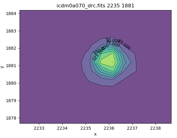
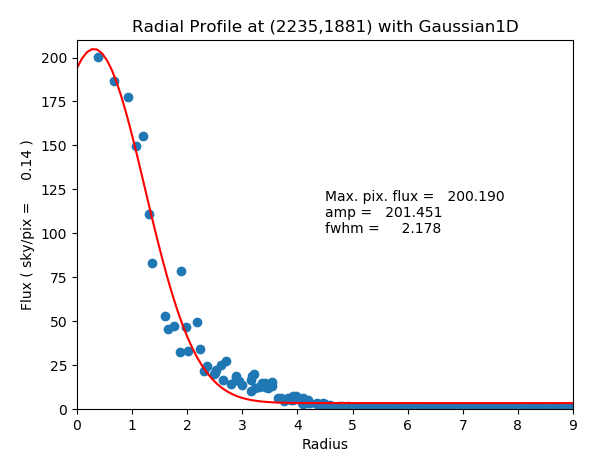
Typing this last command will change the cursor in the ds9 window to a circular, blinking cursor that should be positioned over pixels you wish to analyze. A list of available functions will be displayed in the bash shell, and users who had experience with the previous non-Python imexam will find these functions and their keyboard shortcuts familiar. In Figure 4.2 below, we show plots generated by imexam of the two-dimensional histogram and PSF fit of a star in the drizzled image, which were produced with the keyboard shortcuts "e" and "r", respectively.
Figure 4.2: imexam 2-D Histogram and PSF Fit