5.2 Using Observation Logs

Here are some examples of what can be learned from the observation log files. Some examples assume basic familiarity with FITS file structures and the Python programming language (see Chapters 3 and 4, respectively).

5.2.1 Guide Star Errors

Seldomly, the HST spacecraft pointing may be interrupted during an observation. Subsections 5.2.2 through 5.2.5 describe in detail the information contained within observation log files that can help diagnose the severity of pointing problems and their impact to observations. In general, problems with guide star lock and tracking can be checked using keywords in the "Problem Flags and Warnings" section of the "jif" file primary header. For example, an observation with no loss of guide star lock will have the following in the "jif" file primary header:

              / PROBLEM FLAGS and WARNINGS

T_GDACT =                    T / Actual guiding mode same for all exposures
T_ACTGSP=                    T / Actual Guide Star Separation same in all exps.
T_GSFAIL=                    F / Guide star acquisition failure in any exposure
T_SGSTAR=                    F / Failed to single star fine lock
T_TLMPRB=                    F / problem with the engineering telemetry in any e
T_NOTLM =                    F / no engineering telemetry available in all exps.
T_NTMGAP=                    0 / total number of telemetry gaps in association
T_TMGAP =             0.000000 / total duration of missing telemetry in asn. (s)
T_GSGAP =                    F / missing telemetry during GS acq. in any exp.
T_SLEWNG=                    F / Slewing occurred during observations
T_TDFDWN=                    F / Take Data Flag NOT on throughout observations

These keywords (except T_NTMGAP and T_TMGAP) are Boolean values describing basic tests of pointing quality, and are aggregated from the extensions following the primary extension that describe the individual exposures in the observation/association. Observation logs with deviations from the above may be associated with suspect data, and further examination of the observation logs is warranted.

5.2.2 Guiding Mode

Unless requested, all observations will be scheduled with "FINE LOCK" guiding, which may be one or two guide stars (dominant and roll). The spacecraft may roll slightly during an observation if only one guide star is acquired. The amount of roll depends upon the gyro drift at the time of the observation, the location during an orbit, and the lever arm from the guide star to the center of the aperture.

There are three commanded guiding modes: "FINE LOCK," "FINE LOCK/GYRO," and "GYRO." Observation file header keywords GUIDECMD (commanded guiding mode) and GUIDEACT (actual guiding mode) will usually agree. If there was a problem during the observation, they will not agree and the GUIDEACT value will be the guiding method actually used during the exposure. If the acquisition of the second guide star fails, the spacecraft guidance GUIDEACT may drop from "FINE LOCK" to "FINE LOCK/GYRO," or even to "GYRO," which may result in a target rolling out of an aperture. Check the observation log keywords to verify that there was no change in the requested guiding mode during the observation.

The dominant and roll guide star keywords (GSD* and GSR*) in the observation log header can be checked to verify that two guide stars were used for guiding, or in the case of an acquisition failure to identify the suspect guide star. The dominant and roll guide star keywords identify the stars that were scheduled to be used, and in the event of an acquisition failure may not be the stars that were actually used. The following list of observation log keywords is an example of two-star guiding. These keywords are found in the primary header of the "jif" file in the "Pointing Keywords" section.

              / POINTING CONTROL DATA

GUIDECMD= 'FINE LOCK           ' / Commanded Guiding mode
GSD_ID  = 'N134000416'         / Dominant Guide Star ID
GSD_RA  =           270.236940 / Dominant Guide Star RA (deg)
GSD_DEC =            66.694810 / Dominant Guide Star DEC (deg)
GSD_MAG =            12.649000 / Dominant Guide Star Magnitude
GSD_FGS = '3'                  / Dominant GS Fine Guidance Sensor Number
GSR_ID  = 'N4E8000253'         / Roll Guide Star ID
GSR_RA  =           269.806080 / Roll Guide Star RA (deg)
GSR_DEC =            67.026590 / Roll Guide Star DEC (deg)
GSR_MAG =            13.326000 / Roll Guide Star Magnitude
GSR_FGS = '2'                  / Roll GS Fine Guidance Sensor Number
GS_PRIM = 'ROLL    '           / Guide star that is primary (dominant or roll)
PREDGSEP=             1340.940 / Predicted Guide Star Separation (arcsec)
MGSSPRMS=                   1. / maximum Guide Star Separation RMS in assoc.
TNLOSSES=                    0 / Number of loss of lock events
TLOCKLOS=                   0. / Total loss of lock time
TNRECENT=                    0 / Number of recentering events
TRECENTR=                   0. / Total recentering time

The guide star identifications, GSD_ID and GSR_ID, are different for the two Guide Star Catalogs: GSC2 IDs are 10-characters in length, like those of GSC1, but consist of both letters and numbers. GSC1 IDs consist entirely of numbers.

Some GHRS observations can span several orbits. If during a multi-orbit observation the guide star re-acquisition fails, the observation may be terminated with possible loss of observing time, or switch to other less desirable guiding modes. The GSACQ keyword in the "jif" header will state the time of the last successful guide star acquisition.

GSACQ   = '1997.037:03:45:03 ' /Actual time of GS Acquisition Completion

5.2.3 Guide Star Acquisition Failure

The guide star acquisition at the start of the observation set could fail if the FGS fails to lock onto the guide star. The target may not be in the aperture, or maybe only a piece of an extended target is in the aperture. The jitter values will be increased because "FINE LOCK" was not used. The following list of observation log header keywords in the extensions of the "jif" file corresponding to individual exposures indicate that the guide star acquisition failed.

V3_RMS = 19.3 				  / V3 Axis RMS (milli-arcsec)
V3_P2P = 135.7				  / V3 Axis peak to peak (milli-arcsec)

              / PROBLEM FLAGS, WARNINGS, and STATUS MESSAGES
              /(present only if problem exists)

GSFAIL =  'DEGRADED'		  / Guide star acquisition failure!

The observation logs for all of the exposures in the observation set will have the "DEGRADED" guide star message. This is not a loss-of-lock situation, but an actual failure to acquire the guide star in the desired guiding mode. For the example above, the guiding mode was dropped from FINE LOCK to COARSE TRACK.

GUIDECMD= 'FINE LOCK'		  / Commanded Guiding mode
GUIDEACT= 'COARSE TRACK'	  / Actual Guiding mode at end of GS acquisition

If an observation dataset spans multiple orbits, then the guide star will be re-acquired, but the guiding mode will not change from COARSE TRACK. In September 1995, the flight software was changed so that COARSE TRACK is no longer an option. The guiding mode drops from two guide star FINE LOCK to one guide star FINE LOCK, or to GYRO control.

5.2.4 Moving Targets and Spatial Scans

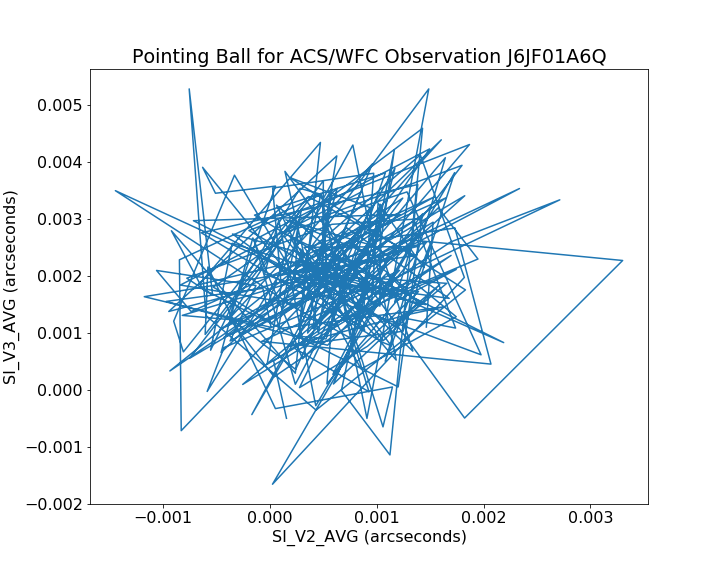
A type 51 slew is used to track moving targets (planets, satellites, asteroids, and comets). Observations are scheduled with FINE LOCK acquisition, i.e., with two or one guide stars. Usually, a guide star pair will stay within the FGS field of view during the entire observation set, but if two guide stars are not available, a single guide star may be used, assuming the drift is small or the proposer says that the roll angle is not important for that particular observing program. An option during scheduling is to drop from FGS control to GYRO control when the guide stars move out of the FGS. Also, guide star handoffs (which are not a simple dropping of the guide stars to GYRO control) will affect the guiding and may be noticeable when the "jitter ball" or "pointing ball" is plotted (see Figure 5.2).

The jitter statistics are accumulated at the start of the observation window. Moving targets and spatial scan motion will be seen in the jitter data and image. Therefore, the observation log keywords V2_RMS and V3_RMS values (the root mean square of the jitter about the V2- and V3-axes¹) can be quite large for moving targets. Also, a special anomaly keyword (SLEWING) will be appended to the observation log header indicating movement of the telescope occurred during the observation. This is expected when observing moving targets. The following list of observation log keywords is an example of expected values while tracking a moving target.

              / LINE OF SIGHT JITTER SUMMARY

V2_RMS  =  3.2       / V2 Axis RMS (milli-arcsec)
V2_P2P  =  17.3      / V2 Axis peak to peak (milli-arcsec)
V3_RMS  =  14.3      / V3 Axis RMS (milli-arcsec)
V3_P2P  =  53.6      / V3 Axis peak to peak (milli-arcsec)
RA_AVG  =  244.01757 / Average RA (deg)
DEC_AVG =  -20.63654 / Average DEC (deg)
ROLL_AVG=  280.52591 / Average Roll (deg)
SLEWING = ‘T’        / Slewing occurred during this observation

5.2.5 High Jitter

The spacecraft may shake during an observation, even though the guiding mode is FINE LOCK. This movement may be due to a micro-meteoroid impact, jitter at a day-night transition, or for some other reason. The FGS is quite stable and will track a guide star even during substantial spacecraft motion. The target may move about in an aperture, but the FGS will continue to track guide stars and reposition the target into the aperture. For most observations, the movement about the aperture during a spacecraft excursion will be quite small, but sometimes, especially for observations with the spectrographs, the aperture may move enough that the measured flux for the target will be less than the previous observation. Check the "jif" header keywords V2_RMS and V3_RMS for the root mean square of the jitter about the V2- and V3-axes. The following list of header keywords, found in the "jif" file, is an example of typical guiding rms values.

              / LINE OF SIGHT JITTER SUMMARY

V2_RMS  = 2.6                  / V2 Axis RMS (milli-arcsec)
V2_P2P  = 23.8                 / V2 Axis peak to peak (milli-arcsec)
V3_RMS  = 2.5                  / V3 Axis RMS (milli-arcsec)
V3_P2P  = 32.3                 / V3 Axis peak to peak (milli-arcsec)

Re-centering events occur when the spacecraft software determines that shaking is too severe to maintain lock. The FGS will release guide star control and within a few seconds re-acquire the guide stars. It is assumed that the guide stars are still within the FGS field of view. During the re-centering time, "INDEF" will be written into the "jit" table. Re-centering events are tracked in the "jif" header file.

Care should be taken when interpreting loss-of-lock and re-centering events that occur at the beginning or at the end of the engineering telemetry window. The telemetry window is larger than the actual observation window. These events might not affect the observation since the observation will start after the guide stars are acquired (or re-acquired), and the observation may stop before the loss-of-lock or re-centering event that occurred at the end of a telemetry window.

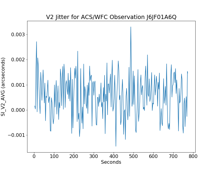
Figure 6.1 shows a plot of the three second time-averaged jitter along the V2-axis of HST for an observation. The Python code used to produce this plot is shown below:

# Imports
from astropy.io import fits
from astropy.table import Table
import matplotlib.pyplot as plt

# Read the data from the jit file into an
# Astropy table
with fits.open('j6jf01a6j_jit.fits') as hdu:
    data = Table(hdu[1].data)
    
# Update the plot font size to 16
plt.rc('font', size=16)

# Plot the data
fig = plt.figure(figsize=(10, 8))
ax = fig.add_subplot(111)
ax.plot(data['Seconds'], data['SI_V2_AVG'])
ax.set_xlabel('Seconds')
ax.set_ylabel('SI_V2_AVG (arcseconds)')
ax.set_title('V2 Jitter for ACS/WFC Observation J6JF01A6Q')

# Save and close the figure
fig.savefig('v2_jitter.png')
plt.close(fig)

Figure 5.1: V2-axis Jitter vs. Time

# Plot the data
fig = plt.figure(figsize=(10, 8))
ax = fig.add_subplot(111)
ax.plot(data['SI_V2_AVG'], data['SI_V3_AVG'])
ax.set_xlabel('SI_V2_AVG (arcseconds)')
ax.set_ylabel('SI_V3_AVG (arcseconds)')
ax.set_title('Pointing Ball for ACS/WFC Observation J6JF01A6Q')

# Save and close the figure
fig.savefig('pointing_ball.png')
plt.close(fig)

Figure 5.2: "Pointing Ball" or V3 jitter vs. V2 jitter in an observation

5.2.6 Spacecraft Information in Observation Logs

More information about the status of the spacecraft and other tracking diagnostics are contained within the observation logs. Here we discuss some of information available.

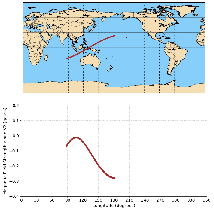
Spacecraft position information and measurements of the magnetic field are contained within the "jit" file data. Below we plot the orbital trace and the magnetic field amplitude in units of Gauss along the V2 axis. The result is shown in Figure 6.3.

from astropy.io import fits
from mpl_toolkits.basemap import Basemap
import matplotlib.pyplot as plt

# Set the font size to 14
plt.rc('font', size=14)

# Read in the jitter file data
with fits.open('icau15esj_jit.fits') as hdu:
    data = hdu[1].data
   
# Set up the figure and subplots
fig = plt.figure(figsize=(10, 10))
ax1 = fig.add_subplot(211)
ax2 = fig.add_subplot(212)

# Create the map projection. This is a cylindrical equidistant projection.
# We have centered the map on longitude 180 degrees, which better suits
# this dataset. We have filled the landmasses with the matplotlib color
# 'wheat' and the water with 'lightskyblue.'
mapproj = Basemap(projection='cyl', lon_0=180, ax=ax1)
mapproj.drawcoastlines()
mapproj.drawcountries()
mapproj.drawparallels(np.arange(-90, 90, 30), alpha=0.1)
mapproj.drawmeridians(np.arange(-180, 180, 30), alpha=0.1)
mapproj.fillcontinents(color='wheat', lake_color='lightskyblue')
mapproj.drawmapboundary(fill_color='lightskyblue')

# Pull the variables we want from the jitter table.
latitude = data['Latitude']
longitude = data['Longitude']
mag_field_v2 = data['Mag_V2']

# Plot the data. Latitude and longitude are plotted on the map,
# while magnetic field strength along V2 is plotted as a function
# of longitude on a subplot below the map.
mapproj.plot(longitude, latitude, lw=4, color='brown')
ax2.plot(longitude, mag_field_v2, lw=4, color='brown')

# Configure the subplot axes and labels.
ax2.set_ylim(-0.4, 0.2)
ax2.set_xlim(0, 360)
ax2.set_xticks(np.arange(0, 361, 30))
ax2.grid(ls=':')
ax2.set_xlabel('Longitude (degrees)')
ax2.set_ylabel('Magnetic Field Strength along V2 (gauss)')

# Reduce whitespace around the plots and save the figure.
plt.tight_layout()
fig.savefig('orbit_magfield.png')
plt.close(fig)

Figure 5.3: HST Orbit and Magnetic Field along V2 Axis

During an exposure, a re-centering event may occur. During these events, the "Recenter" column in the "jit" table will contain a value of 1 (True). During re-centering events and losses of lock, the jitter and pointing data in the observation logs are set to INDEF or 1.6E+38, and these values should be excluded while examining observation logs.

On occasion, the telemetry format stream changes during an observation. During such switches, some engineering data may be lost.

During target acquisition peak-up, the telescope is moved to search for the target in a raster pattern. Once the target is found by the science instrument, the spacecraft automatically moves to center the target. During periods of peak-up, spatial scan, or in the case of a moving target observation, jitter statistics will be incorrect because they will incorporate the motion of the spacecraft.

¹ The V2 and V3 axes are part of the HST V (or ST) coordinate system, which is tied to the HST spacecraft. The V1 axes is the longitudinal axis of the spacecraft. The V2 and V3 axes thus form a plane on which the sky can be projected.