4.6 WFC CCD Detector Charge Transfer Efficiency - CTE
4.6.1 The Issue
The ACS/WFC CCD detectors operate by the simple process of converting incoming photons into electron/hole pairs, collecting the electrons in each pixel. The transfer process moves each pixel's electrons down along the columns and then across in a transfer register to the amplifier located in the corner of the detector array.
When the detectors were manufactured, these transfers were extremely efficient (typically 0.999996 of each charge packet was transferred successfully from one pixel into the next), which means that slightly over 99% of the charge collected in a pixel would be delivered to the transfer register. Once in space, the flux of energetic particles such as relativistic protons and electrons damages the silicon lattice of the CCD detectors. This creates both "hot" pixels and charge traps. This radiation damage is cumulative and was unavoidable given current technologies for detector construction and shielding.
The charge traps degrade the efficiency with which charge is transferred from pixel to pixel during the readout of the CCD array. This is seen directly in the "charge trails" that can extend to over 50 pixels in length upstream (i.e., away from the parallel transfer direction) of hot pixels, cosmic rays and bright stars (see Figure 4.28 for an example).
Figure 4.28: CTE Trails
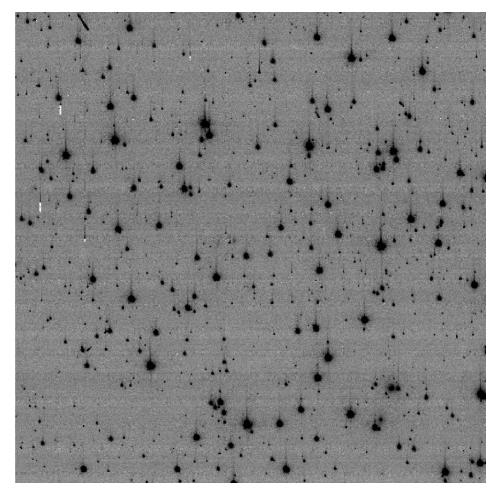
A section (800 × 800) of an ACS frame of 47 Tucanae. Note the presence of parallel CTE trails extending from the stars indicating the effect of CTE on the detector.
4.6.2 Improving CTE: Considerations Before Making the Observations
The simplest mitigation of the imperfect CTE is to reduce the number of charge transfers required for a given source to reach the readout amplifier on the CCD. If the source of interest is small (~10″ across or less), placing it close to the serial register and amplifier will result in greatly enhanced net CTE. APT has a pre-defined aperture setting for this purpose called WFC1-CTE which is located close to the quadrant B amplifier on WFC1.
The CTE loss experienced for a particular pixel's packet of charge depends on the size of the packets that precede it. Larger downstream packets will leave more traps filled and thus unable to grab more charge. This allows more electrons to continue transferring along with the packet. Observations with very low background (< 30 e¯ for ACS) will suffer large losses for very faint sources. This is likely to be problematic for narrow band filters and extremely short exposures. In these cases, raising the background will greatly improve the CTE and thus the S/N of these sources. Users planning to stack multiple images to reach very faint limits should plan to achieve a background level of 30e¯ or more per exposure for ACS. The higher the background level, the higher the percentage of flux above the background survives to readout (See Figure 4 of ACS ISR 2022-04). ACS ISR 2022-04 shows that when the background is 40e- or greater, even the faintest stars retain >50% of their electrons.
The background can be increased in several ways:
- Dividing the total exposure time into fewer, but longer, exposures in order to achieve higher natural backgrounds
- Selection of a broader filter
- Addition of internally generated photons (i.e., "post-flash")
ACS/WFC contains LED lamps configured to illuminate the side of the shutter blade that faces the CCD detector, providing a post-flash capability. While the post-flash lamp can be used to increase the background in an image, users should be cautioned that the post-flash level is not uniform across the detector: it can vary by ~50% from the enter to the corners. See ACS ISR 2014-01 and ACS ISR 2018-02 as well as the ACS website for more details.
4.6.3 Improving CTE: Post-Observation Image Restoration
The ACS team has developed and implemented a post-observation CTE correction algorithm based upon the Anderson and Bedin (2010) methodology. This empirical algorithm is based on a model for charge-transfer loss and release that reproduced the observed trails behind warm pixels. The correction software then uses an iterative forward-modeling process to estimate the source image from the observed trailed image.
The original version of the code worked very well for intermediate to high flux levels (> 200 electrons), but data were not available at the time to set the parameters of the model at lower flux levels. A couple of ISRs describe the original correction: ACS ISR 2011-01 and ACS ISR 2012-03.
In 2018, the pixel-based CTE model was re-parameterized and additional improvements were made. See ACS ISR 2018-04 for details and evaluations of the model's performance with on-sky tests. In 2024, a serial (X-direction) CTE correction model was added to the existing parallel (Y-direction) CTE correction model in CALACS. Serial CTE losses are a minor effect compared to parallel. See ACS ISR 2024-07 for more details.
While pixel-reconstruction algorithms may do a good job removing trails behind stars, cosmic rays, and hot pixels, they have one serious and fundamental limitation: they cannot restore the lost S/N in the image. This limitation notwithstanding, the reconstruction algorithm provides the best understanding of the "original" image before the transfer, and thus gives a sense of how the value of each pixel may have been modified by the transfer process. This algorithm, consisting of both parallel (Y-direction) and serial (X-direction) CTE correction models, is available in the ACS pipeline; standard calibrated products are now available both with and without this correction.
In general, we find that the correction is good to about 25% for stars with moderate signal to noise, so one can get a sense of the reconstruction error by determining the amplitude of the correction and taking 25% of that as the error. ACS ISR 2018-04 provides some empirical demonstrations of the efficacy of the correction.
Degraded CTE is not only an issue for point-sources. ACS ISR 2025-02 examined the impact of degraded CTE on extended sources (of sizes scales ranging from tens to hundreds of pixels) and found measurable flux losses consistent with those seen for point sources, even in FLC/DRC images. While globally measured brightnesses are found to be generally reliable across the detectors as long as standard background recommendations are followed and targets are brighter than 300 e- per exposure, measurements using smaller apertures can be systematically underestimated far from the serial registers.
Figure 4.29: An Example of the Pixel-Based CCD Corrections
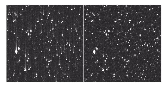
(Left) A 1000 x 1000 pixel region at the top of the chip 1 extension in image jbmncoakq_flt.fits. CTE vertical trails are clearly visible. (Right) The reconstructed CTE-corrected flc.fits image after the execution of calacs.
FLT images. One way to do this is using correction curves and formulae that have been provided in ACS ISR 2022-06. This can be effective for isolated point sources on flat backgrounds, but is less effective for extended sources or sources in crowded regions. Please refer to Section 5.1.5 for more details. Another way to do this is to use the recently released software routine hst1pass (described in ACS ISR 2022-02), which performs PSF-fitting to measure fluxes and positions for point sources in images and can output CTE-corrected fluxes and positions.The expected losses should be taken into consideration when one is deciding on the best CTE-mitigation strategy, which may involve taking fewer longer exposures to preserve S/N even with the increased cosmic-ray contamination.