5.1 Photometry
HRC has been unavailable since January 2007. Information about the HRC is provided for archival purposes.
5.1.1 Photometric Systems, Units, and Zeropoints
It is strongly recommend that, whenever practical, ACS photometric results be referred to a system based on its own filters. Transformations to other photometric systems are possible (see ACS ISR 2019-10 and Sirianni et al. 2005) but such transformations have limited precision and strongly depend on the color range, surface gravity, and metallicity of the stars.
For ACS filters, three magnitude systems are commonly used: VEGAMAG, STMAG, and ABMAG; all of which are based on absolute flux.
The absolute effective flux for any ACS filter and for any Spectral Energy Distribution (SED) can be computed from the throughput for the entire system (OTA + ACS CAMERA + FILTER + DETECTOR) according to Equation 3 of Bohlin et al. (2014).
VEGAMAG is a widely used standard star system, defined as relative photometry to the actual star Vega; Vega magnitudes can be converted to absolute effective fluxes using the flux distribution of this HST secondary standard star1 in the CALSPEC database.
The commonly used photometric systems ABMAG (Oke, J. B. 1964) and STMAG (Koorneef, J. et. al. 1986) are directly related to physical units. The choice between observational and flux-based systems is mostly a matter of personal preference. Any new determination of ACS's absolute efficiency will result in revised magnitudes for these three photometric systems that are based on absolute physical flux.
VEGAMAG
The VEGAMAG system uses Vega (α Lyr) as the standard star. The spectrum of Vega used to define this system is a composite spectrum of empirical and synthetic spectra (Bohlin & Gilliland 2004). The "Vega magnitude" of a star with flux F is
| \mathrm{VEGAMAG} = -2.5\times\log\left(\frac{F}{F_{\mathrm{Vega}}}\right) |
where FVega is the calibrated spectrum of Vega. In the VEGAMAG system, by definition, Vega has zero magnitude at all wavelengths.
STMAG and ABMAG
These two similar photometric systems are also flux-based systems. The conversion is chosen such that the magnitude in V corresponds roughly to that in the Johnson system.
In the STMAG system, the flux density is expressed per unit wavelength, while in the ABMAG system, the flux density is expressed per unit frequency. The magnitude definitions are:
| \mathrm{STMAG} = -2.5\times\log F_\lambda - 21.1 |
| \mathrm{ABMAG} = -2.5\times\log F_\nu -48.60 |
where Fν is expressed in erg cm–2 sec–1 Hz–1, and Fλ in erg cm–2 sec–1 Å–1. Another way to express these STMAG (zero point given by HST header keyword PHOTZPT) and ABMAG zero points of –21.1 and –48.6 is to say that an object with a constant Fν = 3.63 × 10⁻²⁰ erg cm–2 sec–1 Hz–1 will have magnitude AB = 0 in every filter, and an object with Fλ = 3.63 × 10⁻⁹ erg cm–2 sec–1 Å–1 will have magnitude STMAG = 0 in every filter.
Zeropoints
Another sort of zeropoint is the "instrumental zeropoint," which is the magnitude of an object that produces one count per second.
Each zeropoint refers to a count rate measured in a specific aperture. For point source photometry, the measurement of counts in a large aperture is not possible for faint targets in a crowded field. Therefore, counts are measured in a small aperture, then an aperture correction is applied to transform the result to an "infinite" aperture. For ACS, all zeropoints refer to a nominal "infinite" aperture of radius 5".5.
By definition, the magnitude in the passband P in any of the ACS systems (ACSmag(P)) is given by:
| \mathrm{ACSmag}(P) = -2.5\log(\mathrm{e}^-/\mathrm{s}) + \mathrm{ZP}(P) |
The choice of the zeropoint (ZP(P)) determines the magnitude system of ACSmag(P). There are several ways to determine the instrumental zeropoints:
- Use stsynphot to renormalize a spectrum to 1 count/second in the appropriate ACS passband and specify an output zeropoint value based on a selected magnitude system. See the ACS webpage on zeropoints for more details. (Be sure to verify that the most updated throughput tables are being used.) In the following example, a 10,000 K blackbody is renormalized to 1 count/second and the zeropoint for the ACS/WFC F555W filter on the WFC1 CCD is computed on the MJD 57754 (January 1, 2017).
Python INPUT:from astropy import units as u from synphot import SourceSpectrum, Observation from synphot.models import BlackBodyNorm1D import stsynphot as stsyn band = stsyn.band("acs,wfc1,f555w,mjd#57754") spec = SourceSpectrum(BlackBodyNorm1D, temperature=10000) spec_norm = spec.normalize(1 * u.count, band=band, area=stsyn.conf.area) obs = Observation(spec_norm, band) print(obs.effstim("stmag"))
Python OUTPUT:25.657983749640078 mag(ST) (Output may vary slightly due to updates in throughput tables over time.)
- Another equivalent example for finding the STMAG zeropoint for a given filter and observation date can be found in the
- Use values of photometric header keywords (shown below), in the SCI extension(s) of the images, to calculate the STMAG or ABMAG zeropoint:
PHOTFLAMis the inverse sensitivity (erg cm–2 sec–1 Å–1) (electron/s)–1 and represents the flux of a source with constant Fλ, which produces a count rate of 1 electron per second.PHOTPLAMis the pivot wavelength.PHOTZPTis the STMAG zeropoint, permanently set to –21.1.
The header keywords PHOTFLAM, PHOTZPT, and PHOTPLAM relate to the STMAG and ABMAG zeropoints through these formulae (See also Bohlin et al. 2011).
| \mathrm{STMAG\_ZPT} = -2.5\times\log(\mathrm{PHOTFLAM}) - \mathrm{PHOTZPT} = -2.5\times\log(\mathrm{PHOTFLAM}) -21.1 |
| \mathrm{ABMAG\_ZPT} = -2.5\times\log(\mathrm{PHOTFLAM}) -21.10 - 5\times\log(\mathrm{PHOTPLAM}) +18.6921 |
- Use the ACS Zeropoints Calculator; or to calculate them yourself, follow the instructions on the ACS webpage on zeropoints.
The WFC and HRC flux calibrations in terms of new PHOTFLAM values were updated in ACS ISR 2020-08.
5.1.2 Aperture and Color Corrections
In order to reduce errors due to background variations and to increase the signal-to-noise ratio, aperture photometry and PSF-fitting photometry are usually performed by measuring the flux within a small radius around the center of the source. (For a discussion on the optimal aperture size, see Sirianni et al. 2005). However, a small aperture measurement needs to be adjusted to a "total count rate" by applying an aperture correction.
For point sources, ACS zeropoints (available in STMAG, ABMAG, and VEGAMAG) are applied to a measured magnitude that is aperture-corrected to a nominal "infinite" aperture of radius 5.5". The Sirianni paper has been superseded in a number of aspects by Bohlin (2016) and ACS ISR 2020-08, and the revised encircled energy fractions for both a 0.5" and 1.0" aperture from Table 9 of Bohlin (2016) for HRC and from Table 3 of ACS ISR 2020-08 for WFC are reproduced here as Table 5.1. Aperture corrections for the SBC are reported in Table 2 of ACS ISR 2016-05 and use 4" for the "infinite" aperture.
Table 5.1: Encircled Energy Fractions for K Type and Hotter Stars in 0.5" and 1.0" Apertures
Typical formal 1 sigma uncertainties on the 0.5" values are 0.003 for WFC and 0.004 for HRC, while uncertainties for the 1" aperture are 0.001 and 0.003 (Bohlin 2016, ACS ISR 2020-08). For details on how these quantities could vary with time, see Chapter 5.6 in the ACS Instrument Handbook.
FILTER | WFC | HRC | WFC | HRC |
|---|---|---|---|---|
F220W | -- | 0.868 | -- | 0.948 |
F250W | -- | 0.884 | -- | 0.946 |
F330W | -- | 0.898 | -- | 0.943 |
F344N | -- | 0.899 | -- | 0.943 |
F435W | 0.907 | 0.910 | 0.941 | 0.944 |
F475W | 0.911 | 0.914 | 0.943 | 0.946 |
F502N | 0.913 | 0.916 | 0.944 | 0.947 |
F555W | 0.914 | 0.919 | 0.945 | 0.949 |
F550M | 0.914 | 0.920 | 0.945 | 0.949 |
F606W | 0.915 | 0.920 | 0.946 | 0.950 |
F625W | 0.915 | 0.919 | 0.947 | 0.950 |
F658N | 0.916 | 0.917 | 0.948 | 0.949 |
F660N | 0.916 | 0.917 | 0.948 | 0.949 |
F775W | 0.916 | 0.884 | 0.949 | 0.927 |
F814W | 0.914 | 0.862 | 0.949 | 0.910 |
F892N | 0.897 | 0.773 | 0.942 | 0.844 |
F850LP | 0.892 | 0.756 | 0.940 | 0.831 |
Users should determine the aperture correction between their own small-aperture photometry and aperture photometry with a 0.5" radius aperture; this is done by measuring a few bright stars in an uncrowded region of the field of view with both the smaller measurement aperture and the 0.5" radius aperture. The difference between the two apertures should then be applied to all the small aperture measurements. If such stars are not available, small aperture encircled energies have been tabulated by Bohlin (2016). However, accurate aperture corrections are a function of time and location on the chip and also depend on the kernel used by AstroDrizzle2. Blind application of tabulated encircled energies for small radii should be avoided.
Aperture corrections for near-IR filters present further complications because the ACS CCD detectors suffer from scattered light at long wavelengths. These thinned backside-illuminated devices are relatively transparent to near-IR photons; the transmitted long wavelength light illuminates and scatters in the CCD soda glass substrate, is reflected back from the header's metallized rear surface, then re-illuminates the CCDs frontside photosensitive surface (Sirianni et al. 1998). The fraction of the integrated light in the scattered light halo increases as a function of wavelength. As a consequence, the PSF becomes increasingly broad with increasing wavelengths. WFC CCDs incorporate a special anti-halation aluminum layer between the frontside of the CCD and its glass substrate. While this layer is effective at reducing the IR halo, there is a relatively strong scatter along one of the four diffraction spikes at wavelengths greater than 9000 Å (Hartig et al. 2003). See Section 5.1.4 and ACS ISR 2012-01 for more details.
The same mechanism responsible for the variation of the intensity and extension of the halo as a function of wavelength is also responsible for the variation of the shape of the PSF as a function of color of the source. As a consequence, in the same near-IR filter, the PSF for a red star is broader than the PSF of a blue star. Gilliland & Riess (2003) and Sirianni et al. 2005 provide assessments of the scientific impact of these PSF artifacts in the red. The presence of the halo has the obvious effect of reducing the signal-to-noise and the limiting magnitude of the camera in the red and also impacts the photometry in very crowded fields. The effects of the long wavelength halo should also be taken into account when performing morphological studies and performing surface photometry of extended objects. See Sirianni et al. (2005) for more details.
The aperture correction for red objects should be determined using an isolated, same-color star in the field of view, or by using the effective wavelength versus aperture correction relation (Sirianni et al., 2005; ACS ISR 2012-01, Bohlin 2016). If the object's spectral energy distribution (SED) is available, an estimate of the aperture correction is also possible with stsynphot; the parameter aper has been implemented to call the encircled energy tables in the obsmode stsynphot field for ACS. A typical obsmode for an aperture of 0.5" would be specified as "acs,wfc1,f850lp,aper#0.5". A comparison with the infinite aperture magnitude using the standard obsmode "acs,wfc,f850lp" would give an estimate of the aperture correction to apply. Please refer to the stsynphot documentation for more details.
Color Correction
In some cases, ACS photometric results must be compared with existing datasets in different photometric systems (e.g., WFPC2, SDSS, or Johnson-Cousins). Because the ACS filters do not have exact counterparts in any other standard filter sets, the accuracy of these transformations is limited. Moreover, if the transformations are applied to objects whose spectral type (e.g., color, metallicity, surface gravity) do not match the spectral type of the calibration observation, systematic effects could be introduced. The transformations can be determined by using stsynphot, or by using the published transformation coefficients (ACS ISR 2019-10, Sirianni et al. 2005). In any case, users should not expect to preserve the 1%–2% accuracy of ACS photometry on the transformed data.
5.1.3 Pixel Area Maps
When ACS images are flat-fielded by the calacs pipeline; the resultant flt.fits/flc.fits files are "flat" if the original sky intensity was also "flat." However, these flat-fields do not correct for the significant geometric distortion, which causes each pixel to subtend a different angular area on the sky. Therefore, the pixel area on the sky varies across the field, and as a result, relative point source photometry measurements in the flt.fits/flc.fits images will be incorrect.
One option is to drizzle the data; this will remove geometric distortion while keeping the sky flat. Therefore, both surface and point source relative photometry can be performed correctly on the resulting drz.fits/drc.fits files. The inverse sensitivity (in units of erg cm–2 sec–1 Å–1), given by the header keyword PHOTFLAM, can be used to compute the STMAG or ABMAG zeropoint, and to convert flux in electrons/seconds to absolute flux units:
| \mathrm{STMAG\_ZP} = -2.5\log(\mathrm{PHOTFLAM}) - \mathrm{PHOTZPT} |
| \mathrm{ABMAG\_ZP} = -2.5\log(\mathrm{PHOTFLAM}) - 21.10 - 5\log(\mathrm{PHOTPLAM}) + 18.6921 |
where,
- STMAG_ZP is the ST magnitude zeropoint for the observing configuration (given in the header keyword
PHOTMODE). - ABMAG_ZP is the AB magnitude zeropoint for the observing configuration.
PHOTFLAM3 is the mean flux density (in erg cm–2 sec–1 Å–1) that produces 1 count per second in the HST observing mode (PHOTMODE) used for the observation.PHOTZPT3 is the ST magnitude zeropoint (= 21.10).PHOTPLAM3 is the pivot wavelength.
Remember that for point source photometry, one of these zeropoints should be applied to measurements after correcting to the ACS standard 5.5" radius "infinite" aperture.
Additional information about zeropoints is available at the ACS Zeropoints Web page.
Users who wish to perform photometry directly on the distorted flt.fits/flc.fits and crj.fits/crc.fits files, rather than the drizzled (drz.fits/drc.fits) data products, will require a field-dependent correction to match their photometry with that obtained from drizzled data. Only then can the PHOTFLAM and PHOTPLAM values in the flt.fits/flc.fits and crj.fits/crc.fits images be used to obtain calibrated STMAG or ABMAG photometry. (Note: the corresponding drz.fits/drc.fits image has identical PHOTFLAM and PHOTPLAM values.)
The correction to the flt.fits/flc.fits images may be made by multiplying the measured flux in the flt.fits/flc.fits image by the pixel area at the corresponding position using a pixel area map (PAM), and then dividing by the exposure time t. The easiest way to do it is to simply multiply the flt.fits/flc.fits image with its corresponding pixel area map.
| \mathrm{flux}_{\mathrm{DRZ}} = \mathrm{flux}_{\mathrm{FLT}} \times \mathrm{PAM}/\mathrm{t} |
For example, in Python:
from astropy.io import fits
import shutil

shutil.copy('jd1y04rlq_flt.fits', 'jd1y04rlq_fltpam.fits')
flt_hdu = fits.open('jd1y04rlq_fltpam.fits', mode = 'update')
pam1_hdu = fits.open('wfc1_pam.fits')
pam2_hdu = fits.open('wfc2_pam.fits')

flt_hdu['sci', 1].data *= pam2_hdu[0].data
flt_hdu['sci', 2].data *= pam1_hdu[0].data

flt_hdu.close()
pam1_hdu.close()
pam2_hdu.close()
The drz.fits/drc.fits images have units of electrons/seconds, while crj.fits/crc.fits and flt.fits/flc.fits images have units of electrons. The headers of all of these file types have the same PHOTFLAM values.
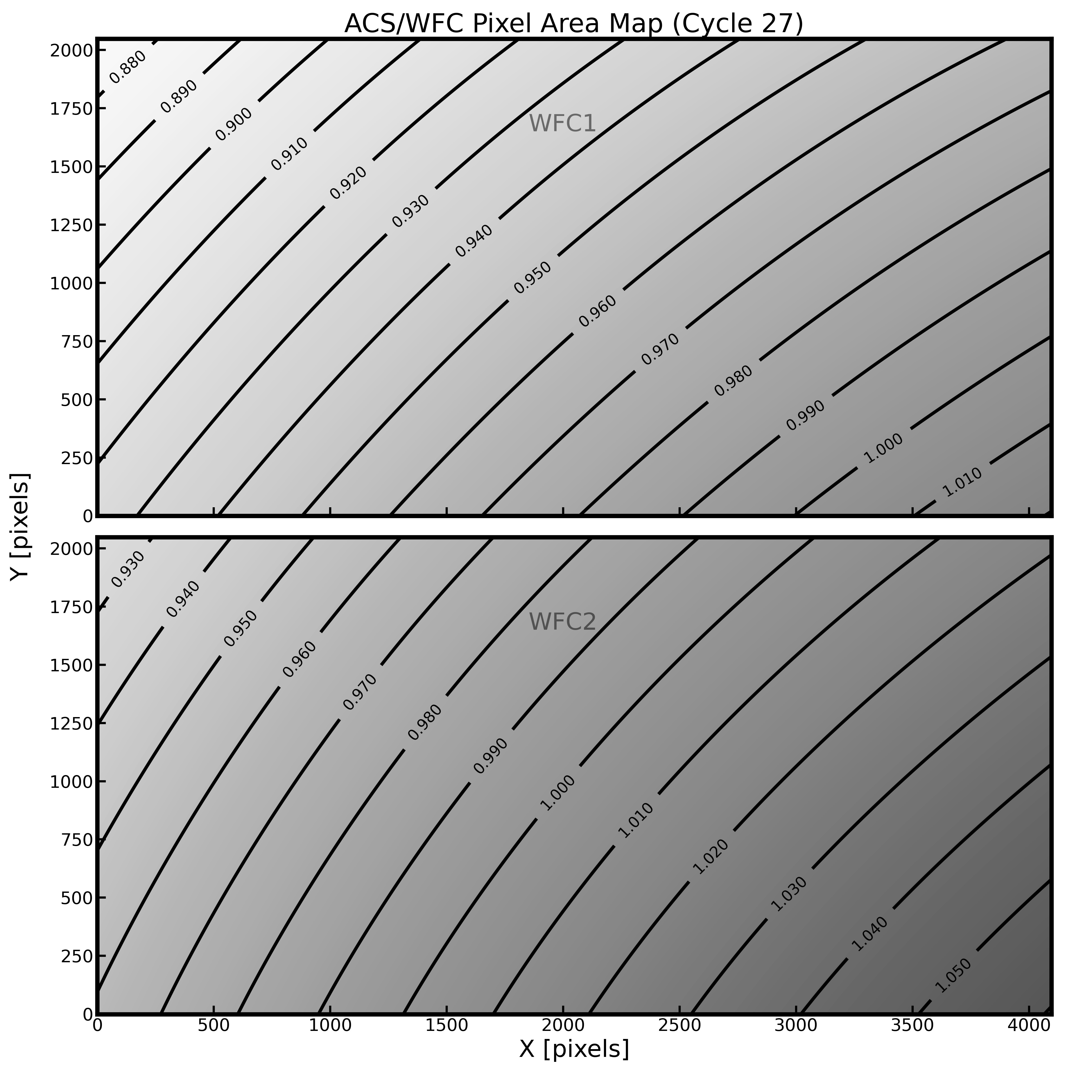
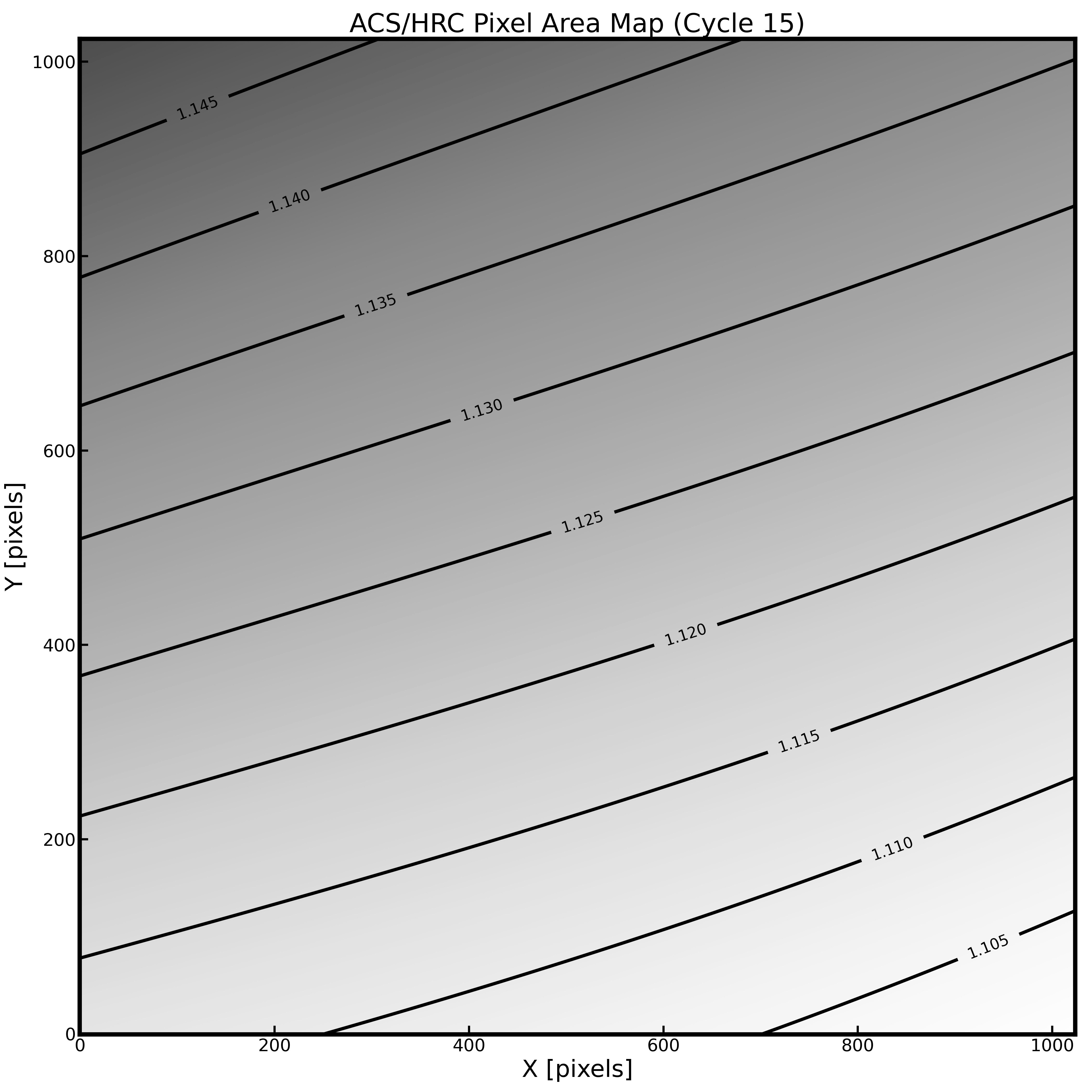
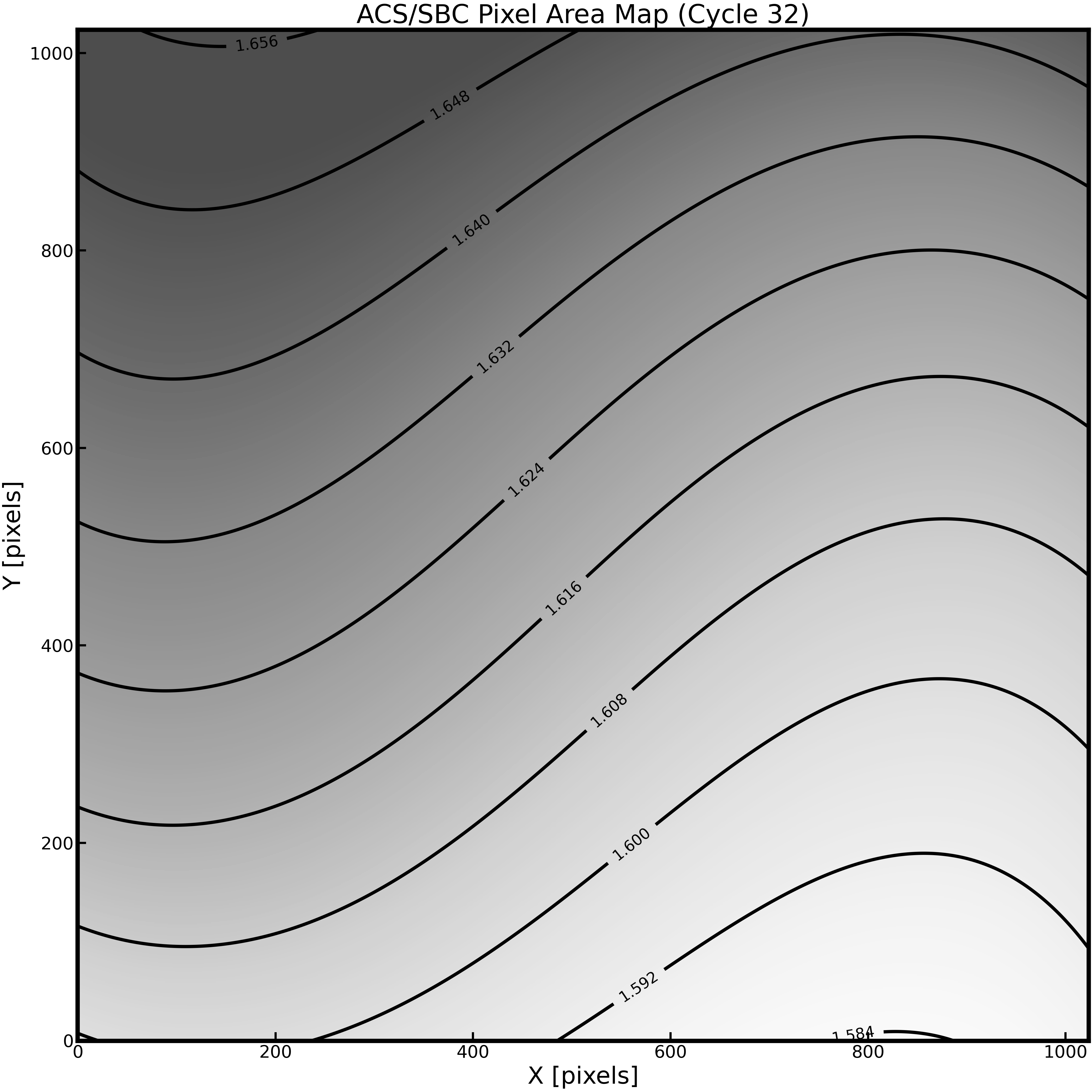
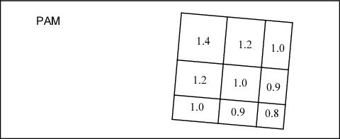
The PAM for the WFC is approximately unity at the center of the WFC2 chip, ~0.95 near the center of the WFC1 chip and ~1.12 near the center of the HRC. Instructions for generating PAMs with pamutils can be found on the Pixel Area Maps ACS webpage. Time-averaged PAM files for the WFC chips and a static PAM for HRC can also be found on that webpage. Note that neither the PAMs generated with pamutils nor the provided PAM files take into account non-polynomial distortion effects tabulated in the NPOLFILE and D2IMFILE.
Figure 5.1: Variation of the WFC, HRC, and SBC Effective Pixel Area with Position in Detector Coordinates
Pixel Area Map Concept Illustration
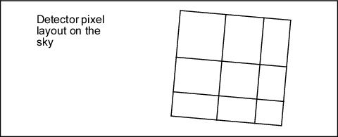
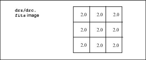
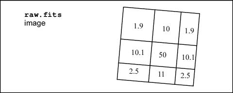
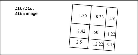
To illustrate the concepts of extended source and point source photometry on flt.fits/flc.fits and drz.fits/drc.fits images, consider a simple idealized example of a 3 × 3 pixel section of the detector, assuming that the bias and dark corrections are zero and that the quantum efficiency is unity everywhere.
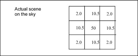
Example #1: Illustration of Geometric Distortion on a Constant Surface Brightness Object
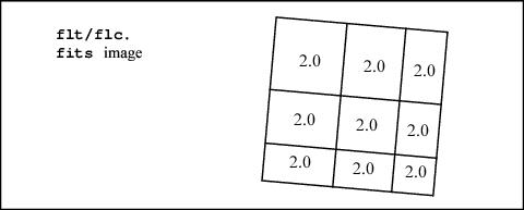
For an extended object with a surface brightness of 2 e¯/pixel in the undistorted case, an image without geometric distortion is:
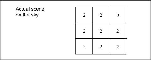
As a result, the raw data shows an apparent variation in surface brightness because some pixels detect flux from a larger sky area than others.

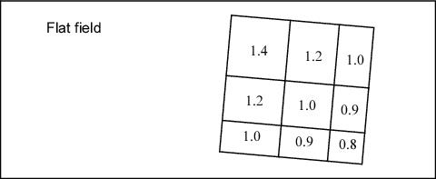
ACS flat fields are designed to produce a flat image when the instrument is uniformly illuminated. This, however, means that pixels which are smaller than average on the sky are boosted, while pixels with relatively large areas are suppressed. Application of the PAM removes this effect—pixels now show the true relative illumination they receive from a uniform source. However, the image remains geometrically distorted. Thus, when doing aperture photometry on the field, the user should take into account that aperture sizes defined in pixels are not uniform in size across the field of view.
If AstroDrizzle is run on a flt.fits/flc.fits image, the output image is free of geometric distortion and is photometrically accurate.
When drizzling a single image, the user may want to use the Lanczos kernel, which provides the best image fidelity for the single image case. However, this kernel does not properly handle missing data and causes ringing around cosmic rays. Thus, the Lanczos kernel should not be used for combining multiple images where sections of the image lost to defects on one chip can be filled in by dithering.
For additional information about the inner workings of AstroDrizzle, please refer to the DrizzlePac website.
Example #2 Illustration of Geometric Distortion and Integrated Photometry of a Point Source
This example considers observing a point source and that all the flux is included in the 3 × 3 grid. Let the counts distribution be:
The total counts are 100. Due to geometric distortion, the PSF, as seen in the raw image, is distorted. The total counts are conserved, but they are redistributed on the CCD, as shown in the fractional area values below.
In this example the counts now add up to 89.08, instead of 100. In order to perform integrated photometry, the pixel area variation needs to be taken into account. This can be done by multiplying the flt.fits/flc.fits image by the PAM or by running AstroDrizzle. Only by running AstroDrizzle can the geometric distortion be removed, but both approaches correctly recover the count total as 100.
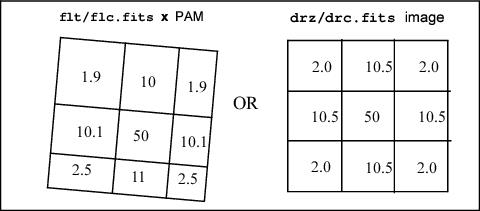
This graphical depiction of geometric distortion and drizzling is just an idealized example. In reality, the PSF of the star extends to a much bigger radius. For photometry radii smaller than 4 pixels, a field-dependent aperture correction must be calculated to avoid photometry errors bigger than 1% (see the next section.) The aperture corrections discussed in Section 5.1.2 are for flt or crj images at the WFC1-1K reference position, as corrected by the PAMs. However, the drz drizzled corrections are the same down to an aperture radius of 3 pixels, where the encircled energy differs by 0.5%.
5.1.4 PSF
PSF Field Dependence
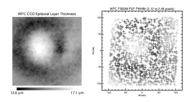
Point spread functions (PSFs) in the ACS cameras are relatively stable over the field of view, especially when compared to previous generation cameras such as WFPC2. Variations in the HRC are very small and probably negligible when using apertures greater than r = 1.5 pixels or using PSF fitting. However, the WFC PSF varies enough in shape and width that significant photometric errors may be introduced when using small apertures or fixed-width PSF fitting. These effects are described in detail in ACS ISR 2003-06.
The WFC PSF width variation is mostly due to changes in CCD charge diffusion. Charge diffusion, and thus the resulting image blur, is greater in thicker regions of the detector (the WFC CCD thickness ranges from 12.6 to 17.1 microns, see Figure 5.2). At 500 nm, the PSF FWHM varies by 25% across the field. Because charge diffusion in backside-illuminated devices like the ACS CCDs decreases with increasing wavelength, the blurring and variations in PSF width will increase towards shorter wavelengths. At 500 nm, photometric errors as much as 15% may result when using small (r < 1.5 pixel) apertures. At r = 4 pixels, the errors are reduced to < 1%. Significant errors may also be introduced when using fixed-width PSF fitting. (See ACS ISR 2003-06).
PSF shape also changes over the WFC field due to the combined effects of aberrations like astigmatism, coma, and defocus. Astigmatism noticeably elongates the PSF cores along the edges and in the corners of the field. This may potentially alter ellipticity measurements of the bright, compact cores of small galaxies at the field edges. Coma is largely stable over most of the field and is only significant in the upper left corner, and centroid errors of ~0.15 pixels may be expected there.
Although TinyTim is no long supported, observers can still use TinyTim to predict the variations in the PSF over the field of view for their particular observation. TinyTim accounts for wavelength and field-dependent charge diffusion and aberrations
For point source relative astrometry, procedures for obtaining the best results are described in ACS ISR 2006-01.
Figure 5.2: WFC Chip Thickness (left) and PSF FWHM (right)
ACS/WFC Focus-Diverse ePSF Tool
The ACS team has put together a focus-diverse effective PSF (ePSF) webtool, available for public access at acspsf.stsci.edu. This tool allows easy access to focus-diverse, effective point-spread functions (ePSFs) for the Wide Field Channel on the ACS instrument. Uneven heating of the telescope’s assembly is known to cause variations in the shape of the PSF, and the empirical ePSF models provided here take this into account. The webtool is automatically updated to include the best-fit focus-diverse ePSFs for new ACS/WFC images every morning. This webtool is based on the initial work in ACS ISR 2018-08 (A. Bellini et al.), and further details can be found in ACS ISR 2023-06 (G. Anand et al.). Updates to the webtool will be advertised in the Change Log at the bottom of the webpage.
PSF Long Wavelength Artifacts
Long wavelength (λ > 700 nm) photons can pass entirely through a CCD without being detected and enter the substrate on which the detector is mounted. In the case of the ACS CCDs, the photons can be scattered to large distances (many arcseconds) within the soda glass substrate before reentering the CCD and being detected—it creates a large, diffuse halo of light surrounding an object, called the "red halo." This problem was largely solved in the WFC by applying a metal coating between the CCD and the mounting substrate that reflects photons back into the detector. Except at wavelengths longer than 900 nm (where the metal layer becomes transparent), the WFC PSF is unaffected by the red halo. The HRC CCD, however, does not have this fix and is significantly impacted by the effect.
The red halo begins to appear in the HRC at around 700 nm. It exponentially decreases in intensity with increasing radius from the source. The halo is featureless but slightly asymmetrical, with more light scattered towards the lower half of the image. By 1000 nm, it accounts for nearly 30% of the light from the source and dominates the wings of the PSF, washing out the diffraction structure. Because of its wavelength dependence, the red halo can result in different PSF light distributions within the same filter for red and blue objects. The red halo complicates photometry in red filters. In broad-band filters like F814W and especially F850LP (in the WFC as well as the HRC), aperture corrections will depend on the color of the star, see Section 5.1.2. for more discussion. Also, in high-contrast imaging where the PSF of one star is subtracted from another (including coronagraphic imaging), color differences between the objects may lead to a significant residual over- or under-subtracted halo.
In addition to the halo, two diffraction spike-like streaks can be seen in both HRC and WFC data beyond 1000 nm (including F850LP). In the WFC, one streak is aligned over the left diffraction spike while the other is seen above the right spike. For HRC, the streak is aligned over the right diffraction spike while the other is seen below the left spike. These seem to be due to scattering by the electrodes on the back sides of the detectors. They are about five times brighter than the diffraction spikes and result in a fractional decrease in encircled energy. They may also produce artifacts in sharp-edged extended sources.
Figure 5.3: CCD Scatter at Red Wavelengths.
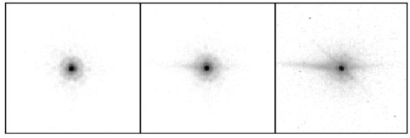
WFC images of the standard star GD71 through filters F775W (9 sec., left), F850LP (24 sec., middle), and FR1016N at 996 nm (600 sec., right). The CCD scatter, undetected below ~800 nm, grows rapidly with longer wavelength. In addition to the asymmetrical, horizontal feature, a weaker diagonal streak also becomes apparent near 1 micron.
HRC and SBC UV PSFs
Below 3500 Å, the low- and mid-spatial frequency aberrations in HST result in highly asymmetric PSF cores surrounded by a considerable halo of scattered light extending 1 to 2 arcseconds from the star. The asymmetries may adversely affect PSF-fitting photometry if idealized PSF profiles are assumed. Also, charge scattering within the SBC MAMA detector creates a prominent halo of light extending about 1" from the star that contains roughly 20% of the light. This washes out most of the diffraction structure in the SBC PSF wings. An updated study of the SBC PSF can be found in ACS ISR 2016-05.
5.1.5 CTE
ACS's WFC and HRC cameras have CCD detectors that shift charge during readout and therefore suffer photometric losses due to imperfect charge transfer efficiency (CTE). Such losses are particularly significant along the parallel direction (y-axis on the detector), and less significant, but present, along the serial direction (x-axis).
Two methods are currently available to correct photometry for CTE losses. The first method uses a pixel-based correction. The second method utilizes a photometric correction formula and may be used to correct photometry of point sources.
Pixel-Based CTE Correction
Anderson and Bedin (2010) developed an empirical approach based on the profiles of warm pixels to characterize the effects of CTE losses for WFC. Such an algorithm first develops a model that reproduces the observed trails, and then inverts the model to convert the observed pixel values in an image into an estimate of the original pixel values. The pixel-based CTE correction, applicable only to full-frame WFC images (CTE-corrected images are not produced for subarrays by the pipeline), has been implemented in the ACS calibration pipeline (calacs). Data products that are corrected for parallel and serial CTE losses have the suffix flc.fits and drc.fits, which correspond to the (uncorrected) flt.fits and drz.fits images. Additional information on the pixel-based CTE correction can be found in Section 4.6.
Photometric CTE Correction
The CTE-correcting formulae described in ACS ISR 2009-01 and ACS ISR 2022-06 can also estimate lost flux as a function of source brightness, sky brightness, x and y position, and time. The pixel-based CTE correction on stellar fields is in general agreement with these photometric correction formulae. Statistically significant deviations are observed only at low stellar fluxes (~300 e¯ and lower) and for background levels close to 0 e¯. For low stellar fluxes, the correction formulae may be more accurate; however, these formulae fail for short exposures with sky values near or below zero, because of the log (sky) or sky to a negative power term.
The formulae are calibrated for conventional aperture photometry with an aperture radius of 3 pixels (3 and 5 pixels for WFC). CTE loss calculations are based on the number of transfers in the y direction that a source undergoes; charge losses that depend on pixel transfers in the x direction are negligible. More details can be found in ACS ISR 2009-01 and ACS ISR 2022-06 for pre- and post-SM4 data, respectively.
CTE Correction Cookbook
This section briefly describes the procedure that users should follow in order to apply the photometric CTE correction formula.
- Obtain
flt.fitsimages using calacs, then use AstroDrizzle to createdrz.fitsdata. Alternatively,drz.fitsfiles from the HST Archive may be used if those images are acceptable. - Multiply the
drz.fitsimages by the exposure time.- For a single exposure
drz.fitsimage, multiply the image by its exposure time. - If the
drz.fitsimage was created from combining severalflt.fitsimages with the same exposure time, multiply thedrz.fitsimage by the exposure time of a singleflt.fitsimage. - If the
drz.fitsfile was made from inputflt.fitsimages with different exposure times, do not use that drizzle-combined image. Instead, run AstroDrizzle to create single exposuredrz.fitsfiles for eachflt.fitsfile. In these situations, the recommended method for photometry is to perform the measurements on each single exposuredrz.fitsimage. Those results can be corrected for CTE losses, then averaged to obtain a more accurate measurement of the stellar flux.
- For a single exposure
- Perform aperture photometry with any preferred software (e.g., photutils). For images drizzled at the native scale, set the photometry aperture radius, r, to 3 pixels. Measure the background for each star locally (e.g., in an annulus of rmin = 13 pixels and rmax = 18 pixels, centered on the star).
- Obtain the epoch of the observation in modified Julian days (MJD) from the header keyword EXPSTART.
- To measure the number of Y-transfers for each star, measure the coordinates of the stars directly on the corresponding
flt.fitsimage. For stars that fall in WFC2 (extension 1 of a multi-extensionflt.fitsfile), the number of transfers, Ytran, is simply the y coordinate of the star. For WFC1, in extension 4 of the same multi-extension FITS file, the number of transfers is Ytran = 2049 – ystar, where ystar is the y coordinate of the star on that frame.
Note the need for particular care in dithered observations. If the position of the star changes only by a few (< 10) pixels, the correction is still well within the error even for large losses. For HRC, Ytran = ystar for readouts with amps C or D, Ytran = 1024 – ystar for readouts with amps A or B.
If the dithers have larger shifts, carefully check the original position of each star in theflt.fitsfiles, then derive the correction using the average value of Ytran. While doing so, it is also recommended to verify that parameters used in AstroDrizzle do not generate any biases when the cosmic ray rejection step is performed—the flux of a star located at different positions on the chip might significantly differ, and AstroDrizzle might interpret such objects as cosmic rays. - Apply the appropriate correction formula (see below) where
- FLUX is the stellar flux measured within the aperture radius (in electrons).
- SKY is the local background for each star (in electrons).
- t is the observation date in modified Julian days.
- Ytran is defined in step 5.
- Apply the magnitude correction to the results of the performed photometry (in magnitudes: magcorrected = magmeasured – Δmag).
- Perform aperture correction. (See Bohlin 2016 and ACS ISR 2020-08).
Any additional corrections (i.e., transforming the flux from e¯ into e¯/sec and applying the zeropoints to transform the flux into AB or Vega magnitudes) should be performed after all of the steps above.
For WFC and pre-SM4 data (MJD < 54129), use the following formula:
\Delta \mathrm{mag} = 10^{A} \times \mathrm{SKY}^B \times \mathrm{FLUX}^C \times (Y_{\mathrm{tran}}/2000) \times (\mathrm{MJD} - 52333)/365 with the following coefficients (and associated 1σ uncertainties): A = –0.14 (0.04), B = –0.25 (0.01), C = –0.44 (0.02).
For WFC and post-SM4 data, users should apply the following formula
\Delta\mathrm{mag_{2000}}(\mathrm{MJD}, \mathrm{F}, \mathrm{SKY}) = a_1 · \log(\mathrm{SKY}) · \mathrm{MJD} · 1/\log(\mathrm{F}) + a_2 · \mathrm{MJD} · 1/(\log(\mathrm{F}))^2 + a_3 · 1/\log(\mathrm{F}) + \\ a_4 · \log(\mathrm{SKY}) · 1/(\log(\mathrm{F}))^2 + a_5 · \log(\mathrm{SKY}) · \log(\mathrm{F}) + a_6 · 1/(\log(\mathrm{F}))^2 + a_7 · \log(\mathrm{F}) + a_8 · \log(\mathrm{SKY}) + a_9
The original coefficients are derived in ACS ISR 2022-06. Updated coefficients are reported on the Photometric CTE Corrections webpage.
Note that the formula for WFC was calibrated using stellar fluxes between ~50 e¯ and ~80,000 e¯ (measured within the 3 pixel aperture radius), and for background levels between ~0.1 e¯ and ~50 e¯. Therefore, to ensure the highest level of accuracy, the formula should be used to correct photometry of stars that are within the range specified above. However, note that for stellar fluxes and background levels higher than the above limits, the amount of the correction is < 2%, even for stars located at the edge of the chip, far from the amplifiers. For very bright stars, the CTE formula currently overestimates CTE losses. For the specific case of very bright stars, the use offlc.fitsanddrc.fits files(i.e., those obtained with the pixel-based CTE correction included in the ACS pipeline) is a better option.
Note that for post-SM4 WFC data, users can utilize the online CTE correction calculator, which also contains a version of this walkthrough.For HRC, the CTE correction can be performed using
\Delta\mathrm{mag} = 10^A \times \mathrm{SKY}^B \times \mathrm{FLUX}^C \times (Y_\mathrm{tran}/1000) \times (\mathrm{MJD} - 52333)/365 with the following coefficients (and associated 1σ uncertainties): A = –0.44 (0.05), B = –0.15 (0.02), C = –0.36 (0.01).
The Relationship Between Field-Dependent Charge Diffusion and CTE
Because the WFC and HRC CCDs were thinned during the manufacturing process, there are large-scale variations in thicknesses of their pixels. Charge diffusion in CCDs depend on the pixel thickness (thicker pixels suffer greater diffusion), so the width of the PSF and, consequently, the corresponding aperture corrections are field-dependent (see Section 5.1.4). ACS ISR 2003-06 characterizes the spatial variation of charge diffusion as well as its impact on fixed aperture photometry. For intermediate and large apertures (r > 4 pixels), the spatial variation of photometry is less than 1%, but it becomes significant for small apertures (r < 3 pixels).
It is unnecessary to decouple the effects of imperfect CTE and charge diffusion on the field dependence of photometry. The CTE correction formulae account for both effects, as long as the user seeks to correct photometry to a "perfect CTE" in the aperture used to obtain measurements (e.g., the recommended aperture radius of 3 pixels). An aperture correction from the measuring aperture to a nominal "infinite" (5.5" radius) aperture is still necessary (see Section 5.1.2).
Internal CTE Measurements
CTE measurements from internal WFC and HRC calibration images have been obtained since the cameras were integrated into ACS. Extended Pixel Edge Response (EPER) and First Pixel Response (FPR) images are routinely collected to monitor the relative degradation of CTE over time. These images confirm a linear degradation with time, but are otherwise not applicable to the scientific calibration of ACS data. Results of the EPER and FPR tests were published in ACS ISR 2005-03 and ACS ISR 2017-01, and are regularly updated on the ACS CTE Information webpage.
5.1.6 Red Leak
HRC
When designing a UV filter, a high suppression of off-band transmission, particularly in the red, had to be traded with overall in-band transmission. The very high blue quantum efficiency of the HRC, compared to WFPC2, made it possible to obtain an overall red leak suppression comparable to that of the WFPC2 while using much higher transmission filters. The ratio of in-band versus total flux, determined using in-flight calibration observations, is given in Table 5.2 for the UV and blue HRC filters, where the cutoff point between in-band and out-of-band flux is defined as the filter's 1% transmission points. This is described in ACS ISR 2007-03. This ISR also reports on the percentage of in-band flux for seven stellar spectral types, elliptical galaxies spectrum (Ell. G), a reddened (0.61 < E(B–V) < 0.70) starburst galaxy (SB), and four different power-law spectral slopes Fλ ~ λα.
Clearly, red leaks are not a problem for F330W, F435W, and F475W and are important for F250W and F220W. In particular, accurate UV photometry of objects with the spectrum of an M star will require correction for the red leak in F250W and will be essentially impossible in F220W. For the latter filter, a red leak correction will also be necessary for K and G types.
Table 5.2: In-band Flux as a Percentage of the Total Flux
O5V | B0V | A0V | F0V | G0V | K0V | M2V | Ell. G | SB | α = –1 | α = 0 | α = 1 | α = 2 | |
|---|---|---|---|---|---|---|---|---|---|---|---|---|---|
F220W | 99.97 | 99.96 | 99.73 | 99.24 | 96.1 | 79.52 | 5.02 | 95.48 | 99.67 | 99.86 | 99.69 | 99.24 | 97.85 |
F250W | 99.98 | 99.98 | 99.8 | 99.71 | 99.42 | 98.64 | 76.2 | 98.15 | 99.82 | 99.93 | 99.87 | 99.74 | 99.45 |
F330W | 99.99 | 99.99 | 99.99 | 99.99 | 99.99 | 99.99 | 99.95 | 99.99 | 99.99 | 99.99 | 99.99 | 99.99 | 99.99 |
SBC
The visible light rejection of the SBC is excellent, but users should be aware that stars of solar type or later will have a significant fraction of the detected flux coming from outside the nominal bandpass of the detector. Details are given below in Table 5.3.
Table 5.3: Visible-Light Rejection of the SBC F115LP Imaging Mode
Stellar Type | Percentage of all Detected Photons which have | Percentage of all Detected Photons which have |
|---|---|---|
O5V | 99.5 | 100 |
B1V | 99.4 | 100 |
A0V | 98.1 | 100 |
G0V | 72.7 | 99.8 |
K0V | 35.1 | 94.4 |
5.1.7 UV Sensitivity
In an ongoing calibration effort, the star cluster NGC 6681 has been observed since the launch of ACS to monitor the UV performance of the HRC and SBC detectors.
Results for the HRC detector for the first year following launch were published in ACS ISR 2004-05. For the three filters, F220W, F250W, and F330W, eight standard stars in the field were routinely measured, indicating a sensitivity loss of not more than ~1% to 2% per year.
Results for the SBC detector have been obtained using repeated measurements of ~50 stars in the same cluster to provide an estimate of the UV contamination in addition to the accuracy of the existing flat fields. The uniformity of the detector response must be corrected prior to investigating any temporal loss in sensitivity. See Section 4.4.2 for a discussion of the SBC flat corrections.
The sensitivity of MAMA detectors declines with time (ACS ISR 2019-04). The sensitivity of the SBC has declined by up to ~10% since launch, with a rate of about 0.5% per year since 2007 (see Figure 5.4). This time-dependent sensitivity requires observation date-dependent zeropoints. The necessary files have been delivered to the calibration pipeline so that the PHOTFLAM header header keyword in SBC images is populated with the correct value. Appropriate zeropoints can also be obtained from the ACS Zeropoints Calculator.
Figure 5.4: Sensitivity of the SBC imaging modes.
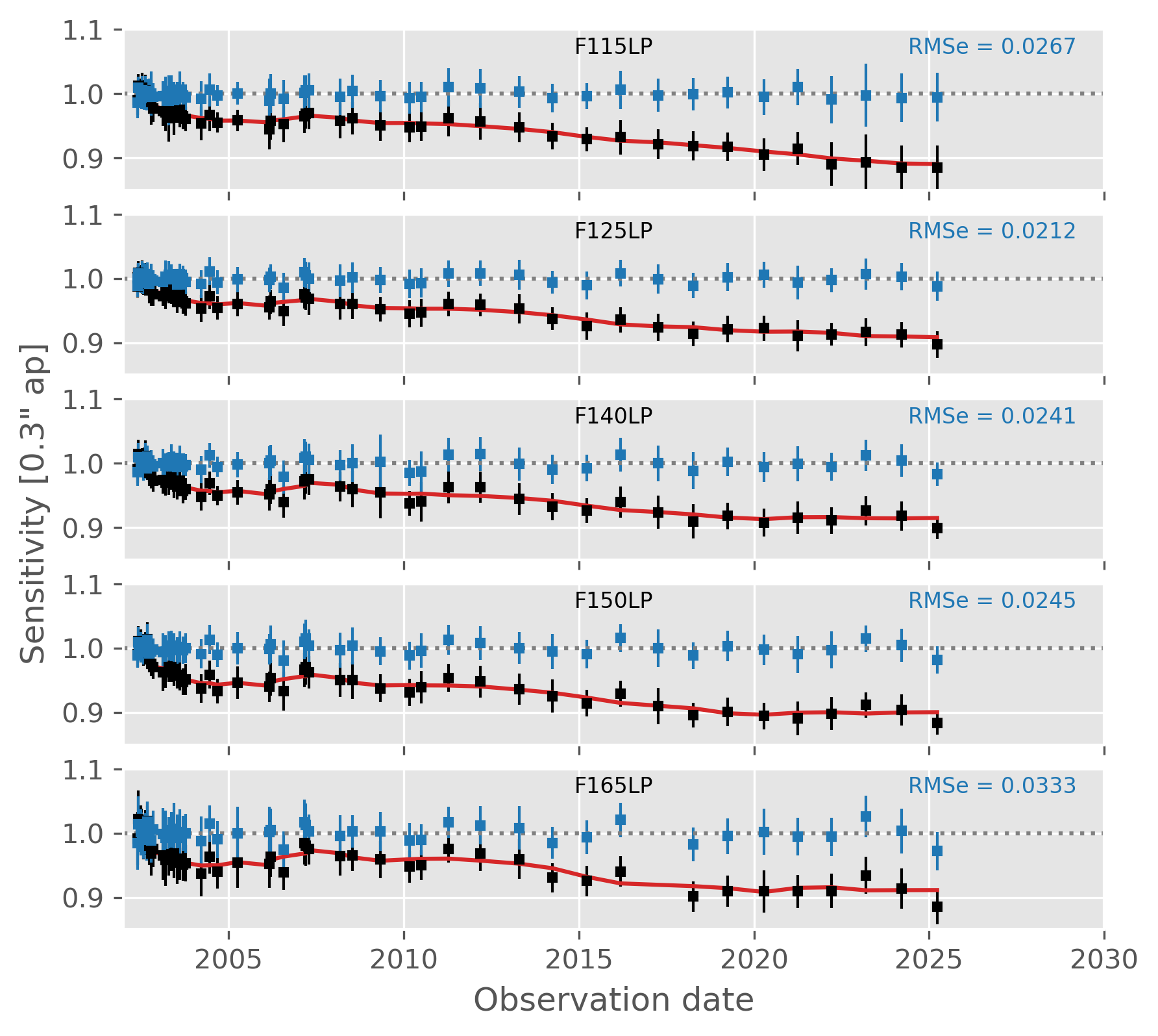
Sensitivity measurements for five SBC imaging modes. Black squares are the mean and standard deviation of the sensitivity before time-dependent sensitivity (TDS) correction. The red line is the extracted TDS. Blue squares are the sensitivity after applying TDS correction.
1 The instrumental flux calibrations are defined by observations of the three primary HST white dwarf (WD) standards GD71, GD153, and G191B2B, which then defines the instrumental sensitivity function for absolute flux. For example, the STIS total throughput sensitivity is used to derive flux distributions for any star observed, including Vega (Bohlin & Gilliland 2004). In other words, the STIS flux for Vega depends only on (1) the absolute fluxes for the three WD primaries, (2) the precision of establishing the STIS calibration from the observations of the three primaries, and (3) the quality of the STIS observations of Vega. Because the HST/STIS Vega flux depends on the flux of other stars, Vega is, by definition, a HST secondary standard except for its monochromatic flux at the one wavelength of 5556 Å which was measured originally relative to tungsten filament lamps. The 5556 Å Vega flux is used to normalize the WD model fluxes distributions via their brightness relative to Vega, as measured by the STIS data. Thus, Vega remains an HST primary star at the one monochromatic wavelength of 5556 Å, making it unique as a sort of hybrid HST secondary/primary star.
2 The final PSF depends slightly on the kernel and pixel scale used to create the output image. This is because the final image is a convolution of the optical/electronic PSF with the final "final_scale" and "final_pixfrac" values. The effect on the PSF is small when the "final_pixfrac" and "final_scale" values are small, and when the measuring aperture is just a few original pixels in radius.
3 Header keyword in calibrated images (flt.fits/flc.fits and drz.fits/drc.fits).
4 STIS ceased science operations in August 2004 due to a power supply failure within its Side-2 electronics (which had powered the instrument since May 2001 after the failure of the Side-1 electronics). In May 2009, during SM4, repairs to the electronics fully restored STIS operation.