5.3 Polarimetry
5.3.1 Absolute Calibration
ACS contains a set of six filters that are sensitive to linear polarization; there are three visible polarizer filters with their polarization directions set at nominal 60° angles to each other, and three UV polarizer filters arranged in a similar manner. The polarizers are aplanatic optical elements coated with Polacoat 105UV (POLUV set) and HN32 polaroid (POLV set). The POLUV set is effective throughout the visible region; its useful range is approximately 2000 Å to 8500 Å. The POLV set is optimized for the visible region of the spectrum and is fully effective from 4500 Å to about 7500 Å. These filters are typically used in combination with a spectral filter which largely defines the spectral bandpass. In most cases observers will obtain images of the target in each of the three filters. The initial calibration steps for polarization data are identical to that for data taken in any other filter—the data are bias-corrected, dark-subtracted, and flat-fielded in the normal manner. The polarization calibration itself is accomplished by combining the set of images (or the resulting counts measured on the images) in the three filter rotations to produce a set of I, Q, and U images, or equivalently, a set of images giving the total intensity, fractional polarization, and polarization position angle.
ACS/WFC polarization data are taken with a 2048 x 2048 subarray. Post-SM4 WFC subarray observations are not de-striped by default, and thus are also not corrected for CTE loss by the data pipeline for storage in MAST. Users wishing to work on de-striped, CTE-corrected data will need to set the PCTECORR flag to PERFORM in the primary header, update the PCTETAB keyword to the correct reference file, and run acs_destripe_plus from the acstools Python package. See the subarray data processing example notebook for assistance.
5.3.2 Instrumental Issues
The design of ACS is far from ideal for polarimetry. Both the HRC and WFC optical chains contain three tilted mirrors and utilize tilted CCD detectors. These tilted components will produce significant polarization effects within the instrument that must be calibrated out for accurate results. There are two primary effects in the tilted components—diattenuation and phase retardance. Diattenuation refers to the fact that a tilted component will likely have different reflectivities (or transmissions) for light that is polarized parallel and perpendicular to the plane of the tilt. This can be an important source of instrumental polarization, and can also alter the position angle of the polarization E-vector. The second effect, phase retardance, will tend to convert incident linear polarized light into elliptically polarized light. These effects will have complex dependencies on position angle of the polarization E-vector, and hence will be difficult to fully calibrate. Additional discussion of these effects can be found in WFPC2 ISR 1997-11, ACS ISR 2004-10, and ACS ISR 2007-10.
The instrumental polarization, defined as the instrument's response to an unpolarized target, provides a simple measure of some of these effects. Figure 5.5 shows the instrumental polarization derived for the HRC through on-orbit observations of unpolarized stars (HST programs 9586 and 9661). The instrumental polarization is approximately 5% at the red end of the spectrum, but rises in the UV to about 14% at the shortest wavelengths. Also shown is a rough model for the effects of the M3 mirror together with a very crude model of the CCD. The mirror is aluminum with a 606 Å thick overcoat of Magnesium Fluoride and has an incidence angle of 47°. Since details of the CCD are proprietary, it has been simply modeled as Silicon at an incidence angle of 31°; no doubt this is a serious over-simplification.
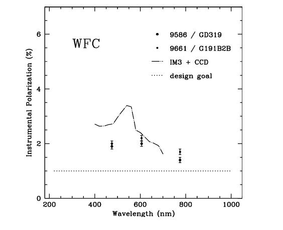
Figure 5.6 shows the same plot for the WFC, which has an instrumental polarization around 2%. Here the IM3 mirror is a proprietary Denton enhanced Silver Coating with an incidence angle of 49°, and the CCD has an incidence angle of 20°. While the lower instrumental polarization of the WFC seems attractive, users are cautioned that the phase retardance effects are not known for the Denton coating, and have some potential to cause serious problems—if sufficiently large, the retardance could produce a large component of elliptical polarization which will be difficult to analyze with the linear polarizers downstream.
Figure 5.5: Instrumental Polarization for the HRC
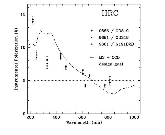
Figure 5.6: Instrumental Polarization for the WFC
One further issue for polarizer data is added geometric distortion. The polarizers contain a weak lens which corrects the optical focus for the presence of two filters in the light path. The lens causes a large scale distortion that appears to be well-corrected by the drizzle software. There is also, however, a weak (±0.3 pixel) small scale distortion in the images caused by slight ripples in the polarizing material. There is presently no correction available for this. There is also the possibility of polarimetric field dependences; while there has been study of intensity flats for the polarizers, the polarization field dependencies are not known.
5.3.3 Flats
Flat fields for the ACS polarizers were obtained in the laboratory and corrected for low frequency variations using the in-flight L-flat corrections which were derived for the standard (non-polarizer) filters. The pivot wavelength of the combined optical components is typically within 1% when the standard filters are used in combination with the polarizers instead of with the clear filters. To assess the accuracy of this approximation, in-flight observations of the bright Earth using the F435W+POLUV filters were compared with the F475W+POLV filters with the corrected laboratory flats. The HRC Earth flats agreed with the corrected lab flats to better than 1%, where the largest deviations occurred near the edges of the detector.
5.3.4 Polarization Calibration
An extensive series of on-orbit polarization calibration observations were carried out in Cycles 11 and 12 (programs 9586, 9661, and 10055). These included observations of unpolarized and polarized standard stars, the star cluster 47 Tuc, and an extended reflection nebula. Additional observations of polarized standards were taken over a wide and well-sampled range of HST roll angles to help quantify the angular dependences which are expected as the wavefront interacts with the diattenuation and phase retardation in the mirrors and CCD.
These calibrations, based largely on data in programs 9586 and 9661, are available for use by polarization observers. The number of polarimetric observations obtained with ACS is very small compared to other modes. As a result of this, the polarimetric mode has not been calibrated as precisely as other modes because of limited resources. For details, please see ACS ISR 2007-10 and also Hines et al. (2014), which contains the most up-to-date coefficients for the F606W filter.
The ACS Team is currently working to improve the calibration of the polarizers using data from two programs (13964 and 14407). Updates will be posted on the ACS website. This calibration can be applied to either aperture photometry results, or to the images themselves (i.e., for an extended target).
The calibration process began with the polarization "zeropoint" using corrections which were derived from observations of unpolarized standard stars.
An update to the acstools Python package in December 2020 adds the polarization_tools module that provides conveniences for the following equations and calibration coefficients. Astropy table versions of the efficiency corrections (Table 5.6) and cross-polarization leak terms (Table 5.7) are included for convenience. An example notebook demonstrating the basic functionality of the polarization_tools module is available.
Efficiency corrections C(\mathrm{CCD}, \mathrm{POLnXX}, \mathrm{spectral\ filter}, n) need to be applied to the observed count rate r_{\mathrm{obs}, n} in each of the three polarizers (POLnUV or POLnV, where n = 0, 60, 120), before the images are used to form the Stokes parameters. These corrections are tabulated in Table 5.6, and have been scaled such that Stokes I will approximate the count rate seen with no polarizing filter.
| r_n = C(\mathrm{CCD}, \mathrm{POLnXX}, \mathrm{spectral\ filter}, n) r_{\mathrm{obs}, n} |
Next, an "instrumental" Stokes vector is computed for the target.
| I = \dfrac{2}{3}\left(r_0 + r_{60} + r_{120}\right)\\ Q = \dfrac{2}{3}\left(2r_0 - r_{60} - r_{120}\right)\\ U = \dfrac{2}{\sqrt{3}}\left(r_{60} - r_{120}\right) |
Next, the fractional polarization of the target is computed, P. Also included is a factor that corrects for cross-polarization leakage in the polarizing filters (see Table 5.7 for the average correction factor per filter for a spectrum flat in wavelength).
| P = \dfrac{\sqrt{Q^2 + U^2}}{I} \times \left[\dfrac{T_{\mathrm{par}} + T_{\mathrm{perp}}}{T_{\mathrm{par}} - T_{\mathrm{perp}}}\right] |
Finally, the position angle on the sky of the polarization E-vector is computed. The parameter PAV3 is the roll angle of the HST spacecraft, and is found in the header keyword PA_V3. The parameter \chi contains information about the camera geometry which is derived from the design specifications; for HRC, \chi = –69.4°, and for the WFC, \chi = –38.2°. Note that the arc tangent function must be properly defined; here, the result is defined as positive in quadrants I and II, and negative in III and IV.
| \theta = \dfrac{1}{2}\tan^{-1}\left(\dfrac{U}{Q}\right)+\mathrm{PAV3} + \chi |
For example, a target that gives 65192, 71686, and 66296 counts per second in the HRC with F606W and POL0V, POL60V, and POL120V, respectively, is found to be 5.9% polarized at PA = 96.9°.
The full instrumental effects and the above calibration have been modeled together in an effort to determine the impacts of the remaining uncalibrated systematic errors. These will cause the fractional polarizations to be uncertain at the one-part-in-ten level (e.g., a 20% polarization has an uncertainty of 2%) for highly polarized sources; and at about the 1% level for weakly polarized targets. The position angles will have an uncertainty of about 3°. (This is in addition to uncertainties that arise from photon statistics in the observer's data.) This calibration has been checked against polarized standard stars (~5% polarized) and found it to be reliable within the stated errors. Better accuracy will require improved models for the mirror and detector properties as well as additional on-orbit data. No calibration has been provided for F220W, F250W, or F814W, as they are believed to be too unreliable at this time. There is also some evidence of a polarization pathology in the F625W filter, and observers should be cautious of it until the situation is better understood. In addition, one incidence of a 5° PA error for F775W has been observed, suggesting this waveband is not calibrated as well as the others. Better characterization of the F775W filter is on-going.
Table 5.6: Efficiency Correction Factors C(CCD, POLnXX, specfilt, n) for Polarization Zeropoint
CCD | POL Filter | Spectral Filter | n = 0 | n = 60 | n = 120 |
|---|---|---|---|---|---|
HRC | POLUV | F330W | 1.7302 | 1.5302 | 1.6451 |
| POLV | F435W | 1.6378 | 1.4113 | 1.4762 | |
POLV | F475W | 1.5651 | 1.4326 | 1.3943 | |
| POLV | F606W | 1.4324 | 1.3067 | 1.2902 | |
| POLV | F625W1 | 1.0443 | 0.9788 | 0.9797 | |
| POLV | F658N1 | 1.0614 | 0.9708 | 0.9730 | |
| POLV | F775W | 1.0867 | 1.0106 | 1.0442 | |
WFC | POLV | F475W | 1.4303 | 1.4717 | 1.4269 |
| POLV | F606W | 1.2960 | 1.3238 | 1.2781 | |
| POLV | F775W | 0.9965 | 1.0255 | 1.0071 |
1 Not scaled for Stokes I
Table 5.7: Flat-Spectrum (with Wavelength) Average Cross-Polarization Leak Correction Factors
| CCD | POL Filter | Spectral Filter | Tparallel | Tperpendicular | Leak Correction |
|---|---|---|---|---|---|
| HRC | POLUV | F330W | 0.4810 | 0.0470 | 1.2167 |
| POLUV | F435W | 0.5247 | 0.0416 | 1.1724 | |
| POLV | F606W | 0.5158 | 5.591 x 10⁻⁵ | 1.0002 | |
| POLV | F625W | 0.5147 | 2.874 x 10⁻⁵ | 1.0001 | |
| POLV | F658N | 0.5174 | 2.355 x 10⁻⁵ | 1.0001 | |
| POLV | F775W | 0.6043 | 0.0732 | 1.2758 | |
| WFC | POLV | F475W | 0.4239 | 1.524 x 10⁻⁴ | 1.0001 |
| POLV | F606W | 0.5157 | 5.591 x 10⁻⁵ | 1.0002 | |
| POLV | F775W | 0.6041 | 0.0737 | 1.2778 |
5.3.5 Imaging Spectropolarimetry
As discussed in the ACS Instrument Handbook, the polarizers can be paired with the G800L grism to obtain imaging spectropolarimetry with spectral resolving power (R~100 @ 8000Å) from ~5500Å – 8000Å. Commissioning and characterization of this mode in Cycle 30 indicates that this new mode will be capable of measuring polarization signals with precision in percentage polarization ~1-2%, and with similar absolute accuracy. Because this mode is slitless, it is most suited for point-sources. However, slightly extended sources up to 2-3 arcseconds have been observed as polarization calibrators during the commissioning process, and reliable results should still be obtained for such objects with intrinsic polarizations >~ 4-8%. Note that polarization follows a Rice as opposed to a Poisson distribution, so confident polarization measurements require an absolute minimum P/σp > 4; however, 5 is the highly recommended minimum. Spaxels may be binned to achieve this requirement, if necessary, but at the expense of spatial and spectral resolution.
The general procedures for obtaining Stokes parameters follows the prescription above. However, there are a important differences to properly construct the Stokes parameters for the Imaging Spectrpolarimetry mode. In particular, the polarizing efficiency corrections and cross-polarization leak factors in Tables 5.6 and 5.7 are not used, because this information is contained in a polarizing efficiency spectrum that is applied at the end of processing. The file is multiplied into the POLV 2D images just prior to the formation of the Stokes Q and U parameters. This correction is still being characterized, so observers reducing spectropolarimetry data should contact the Help Desk for the most up-to-date information.
It is crucial for proper polarimetry reduction that all steps be performed in 2D space until the very end when a 1D spectrum can be extracted (if that is the end goal).
For each triple set of observations (G800L+POL0V, G800L+POL60V, G800L+POL120V)
- Apply distortion corrections — done with AstroDrizzle with EXP weighting (the resulting images must be in units of e-/s)
- Align images – this alignment needs to be more accurate than just using the WCS – use zeroth order or a star in the field
- Form Stokes parameters, Q and U, and also P and θ using the prescription above, but do not apply the transmission correction term
- Apply the polarization efficiency correction file
- Extract Q, U, P and θ spectra as needed using the standard ACS grism extraction software (currently, HSTaXe)
In some circumstances, observers may wish to combine data from multiple visits. This may happen when observers use a different roll angle on the telescope to help separate overlapped spectra. In these cases, it is crucial that the co-additions are performed in Q and U space, not in P and θ space. The fractional polarization (P) follows a Rice distribution, not a Poisson distribution, so co-addition in P-space will yield erroneous results.
Observers should examine the 2D images in Q and U (or in P and θ) to look for stars in the field. Most stars in the galaxy have low or zero polarizations. Therefore, the field stars should all be unpolarized and have Q = U = P = 0. Polarization signals in field stars may indicate a problem with the calibration. Unless observers know in advance that the stars in the field are polarized, they should contact the Help Desk for guidance.
After the primary reductions have been completed, main Stokes parameters (I, Q, U) should be in count-rate units (e-/s). Observers wanting to manipulate Stokes parameters for plotting in Stokes diagrams, for example, should consider using the normalized Stokes parameters q = Q/I and u = U/I. This removes any issues related to absolute flux density calibrations, which are still being derived. The ACS team will provide absolute calibration conversion spectra for Q, U, and I in the future. For the near term, the Stokes parameter (I) can be calibrated using current G800L flux calibration files between 4500Å - 8000Å. For longer wavelengths, the intensity Stokes parameter (I) is not properly given by the equation above, and approaches 0.5*(I) from that formula. This is because the polarizing efficiency rapidly approaches zero for longer wavelengths; the total intensity can still be used and calibrated, but polarization measurements are not possible for wavelengths >8000Å.
The ACS Instrument Team emphasizes that this is a newly commissioned mode, and is still being fully characterized and calibrated. Observers using this mode should contact the Help Desk to initiate a dialog with the team.