5.6 Spectroscopy with the ACS Grisms and Prisms
The ACS WFC has a grism (G800L) which provides slitless spectra at a dispersion of ~40 Å/pixel in the first order over the whole field of view. The same grism, used with the HRC, produced higher dispersion spectra (~23 Å in first order).
A prism (PR200L) available with the HRC provided slitless spectra from the UV cut-off to ~3500 Å.
The SBC is fitted with two prisms (PR110L and PR130L) which provide far-UV spectra, the latter blocked below 1230 Å to prevent transmission of Lyman α.
All of the ACS spectroscopic modes present the well-known advantages and disadvantages of slitless spectroscopy. The chief advantage is area coverage enabling spectroscopic surveys. Among the disadvantages are overlap of spectra, high background from the integrated signal over the passband and modulation of the resolving power by the sizes of dispersed objects. For ACS, the low background from space and the narrow PSF make slitless spectra competitively sensitive to ground-based spectra from larger telescopes in the presence of sky background.
The primary aim of reduction of slitless spectra is to provide one-dimensional wavelength and flux calibrated spectra of all the objects with detectable spectra. The reduction presents special problems on account of the dependence of the wavelength zero point on the position of the dispersing object, the blending of spectra in crowded fields, and the necessity of flat fields over the whole available wavelength range. For ACS slitless modes, a dedicated package was developed by the ST-ECF to enable automatic and reliable extraction of large numbers of spectra. This package, called aXe, is sufficiently general to be used for other slitless spectra applications. A separate software package, HSTaXe, which is a PyRAF-independent follow-up to aXe, can now be used to extract and calibrate spectra from ACS grism exposures. Additional information is available at the aXe/HSTaXe website. Recently, the ACS team produced a new python package (Slitlessutils) to extract and simulate slitless spectroscopy. For spectral extraction, the package offers two techniques: the single-orient extraction, which employs a very similar algorithm to aXe, while the multi-orient extraction enables the linear-reconstruction techniques developed by Ryan, Casertano, & Pirzkal (2018). Although this package is under active development, the current stable versions are on GitHub, with more information available in the package's documentation.
5.6.1 What to Expect from ACS Slitless Spectroscopy Data
The default method for taking ACS slitless spectra is to take a pair of images, one direct and one dispersed, in the same orbit (using special requirement AUTOIMAGE=YES1 in APT, see the HST Phase II Proposal Instructions for details). Or, at the least, to take them with the same set of guide stars and without a shift in-between imaging and spectroscopic observations. The filter for the direct image is set by the AUTOIMAGE=YES parameter. Alternately, a direct image using a filter in the range of the spectral sensitivity can be explicitly specified in the exposure logsheet; in that case, AUTOIMAGE should be set to "NO." For ACS/WFC G800L observation, this latter method is preferred and it is recommended that observer choose the F775W filter (as it is closest to the midpoint of the G800L grism) to minimize filter shifts. When setting up the Phase II Proposal, it is also recommended to contain these pair of observations in a Exposure Sequences Container to ensure these two observations are taken one after another without interruptions. See Chapter 4 Visits, Exposures, and Exposure Groups in the HST Phase II Proposal Instructions for details.
The direct image provides the reference position for the spectrum and thus sets the pixel coordinates of the wavelength zero point on the dispersed image. The adequacy of the direct image to provide the wavelength zero point can be assessed by checking the WCS of the direct and dispersed images. In general this can be trusted at the level of a pixel or better. Detailed information about the pointing during an observation can be obtained from the jitter files.
In the case of a direct image not being available, such as when the pairing of a dispersed image with a direct image was suppressed (AUTOIMAGE=NO), then it is possible, for G800L grism observations, to use the zeroth order to define the wavelength zero point. However the detected flux in the zeroth order is a few percent of that in the first order and it is dispersed by about 5 pixels, so the quality of the wavelength information will be degraded.
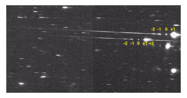
As an example, Figure 5.7 shows an ACS image (one chip only) taken with F775W and Figure 5.8 shows the companion G800L dispersed image. This illustrates the general characteristics of slitless spectra and the characteristics of ACS spectra in particular.
Figure 5.7: Direct Image of WFC1 in F775W
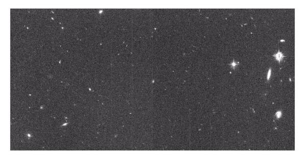
Figure 5.8: WFC1 G800L Slitless Image Corresponding to the Direct Image. The yellow numbers indicate the different grism orders (-2,-1,0,+1,+2).
Bright Stars
The brightest objects produce spectra which can extend far across the chip. For the G800L grism, only about 10% of the flux is in orders other than the first, but for bright objects, orders up to +4 and –4 can be detected. These spectra, while in principle can be analyzed2, are a strong source of contamination for fainter spectra. In addition, for the grism, higher order spectra are increasingly out of focus and thus spread in the cross-dispersion direction.
In the case of the prisms, the strongly non-linear dispersion can result in heavily saturated spectra to longer wavelengths. An additional effect for bright stars is the spatially extended spectra formed by the wings of the PSF.
Resolution and Object Size
In slit-based spectroscopy, the size of the aperture (e.g. slit width) becomes a relevant size scale in determining the spectral resolution: higher resolution is achieved for narrower slit widths. However, slitless spectroscopy has no slit, and so the finite size of the object (projected along the dispersion axis) becomes the relevant size scale. Therefore, large, extended sources will have lower spectral resolution than smaller compact ones. The ACS PSF has a high Strehl ratio for most channels and accessible wavelengths, therefore point sources achieve nearly the theoretical resolution (see ACS ISR 2001-02).
Zeroth Order
The grism zeroth order, only detectable for brighter objects since it contains about 3% of the total flux, can be mistaken for an emission line. The direct image can be used to determine the position of the zeroth order, and for brighter sources, distinguish unequivocally between the zeroth order and an emission line. It is worth noting that the zeroth order is itself dispersed (albeit very much shorter compared to the first order) so it is not same as the direct image and it is not at the same position as the direct image. Because of the dispersed nature of the zeroth order spectra, it is difficult to centroid the location of the source using the zeroth order. Using the location of the zeroth order as the wavelength zero point is thus not recommended and the preferred method is use the location of the source in the direct image, taken before the dispersed image were taken.
Background
The background in a single pixel is the result of the transmission across the whole spectral range of the disperser and can thus be high depending on the spectrum of the sky background. The SBC PR130L prism, for example, provides lower detected background than the PR110L since it excludes the geocoronal Lyman α line. Bright objects in the field elevate the local background both in the dispersion direction and in the cross-dispersion direction. This background needs to be carefully removed before or after extracting the spectra of targets.
Crowding
Although Figure 5.7 and Figure 5.8 show a relatively uncrowded field, close examination shows many instances where spectra overlap, either in the dispersion direction or between adjacent spectra. It is important to know if a given spectrum is contaminated by a neighbor. To resolve the contamination from unassociated neighboring objects, one has a few options: 1) provide a detailed estimate for the spectrum of the sources (such as coming from aggregate broadband photometry) to improve the contamination modeling in HSTaXe/aXe with the FLUXCUBE formalism, 2) rotate the telescope such that two objects no longer overlap, and/or 3) employ the linear reconstruction techniques of Ryan, Casertano, Pirzkal (2018).
Extra Field Objects
There will inevitably be cases of objects outside the field which produce detectable spectra. This is more serious for the HRC and SBC where the fields are small and the spectra are long relative to the size of the detector. In such cases reliable wavelengths cannot be assigned since the zero point of the wavelength scale cannot be determined unless the zeroth order is also present. Brighter sources are a source of contamination, and correct flagging is hampered by the lack of knowledge of the precise image position.
5.6.2 Pipeline Calibration
The direct image obtained before a grism-dispersed observation is fully reduced by calacs in the pipeline. However, the only pipeline steps applied to a dispersed image involve noise and data quality array initializations, linearity corrections for the SBC, and for the CCDs, bias subtraction, dark correction, removal of the image overscan areas, and sink pixel flagging (if the data were taken after Jan 1, 2015). The grism-dispersed images are also flat-fielded using a placeholder (dummy) flat field during this step, and the data units are converted to electrons (which includes gain conversions for the CCDs3). Table 5.7 shows the calibration switches appropriate for a WFC G800L frame.
A placeholder (dummy) flat, filled with the value "1" for each pixel, is used because no single flat-field image can be correctly applied to slitless spectroscopy data, since each pixel cannot be associated with a unique wavelength. Rather, flat-fielding is applied later during the extraction of spectra using an aXe/HSTaXe task called aXe_PETFF (see Section 5.6.4). Each pixel receives a flat-field correction dependent on the wavelength falling on that pixel as specified by the position of the direct image and the dispersion solution. No unique photometric keywords can be attached to all the spectra in a slitless image, so the photometric header keywords are left as default values as shown in Table 5.8.
For all subsequent reductions of slitless data using aXe/HSTaXe, the pipeline flt.fits/flc.fits files should be the starting point.
Table 5.7: Calibration Switch Settings for an Individual ACS WFC Slitless Spectroscopy Frame
Keyword | Switch | Description |
|---|---|---|
STATFLAG | F | calculate statistics? (T/F) |
WRTERR | T | write out error array extension? (T/F) |
DQICORR | PERFORM | data quality initialization? |
ATODCORR | OMIT | correct for A to D conversion errors? |
BLEVCORR | PERFORM | subtract bias level computed from overscan image? |
BIASCORR | PERFORM | subtract bias image? |
FLSHCORR | OMIT | subtract post-flash image? |
CRCORR | OMIT | combine observations to reject cosmic rays? |
EXPSCORR | PERFORM | process individual observations after cr-reject? |
SHADCORR | OMIT | apply shutter shading correction? |
DARKCORR | PERFORM | subtract dark image? |
FLATCORR | PERFORM | apply flat field correction? |
PHOTCORR | OMIT | populate photometric header keywords? |
RPTCORR | OMIT | add individual repeat observations? |
DRIZCORR | PERFORM | process dithered images? |
SINKCORR | OMIT | flag sink pixels? (PERFORM IF WFC data with date > Jan 1 2015) |
Table 5.8: ACS Slitless Spectra (Grism or Prism) Photometric Keywords
Keyword | Value | Description |
|---|---|---|
PHOTMODE | 'ACS WFC2 G800L' | observation con |
PHOTFLAM | 0.00000E+00 | inverse sensitivity, ergs/cm2/Ang/electron |
PHOTZPT | 0.00000 | ST magnitude zero point |
PHOTPLAM | 0.00000 | Pivot wavelength (Angstroms) |
PHOTBW | 0.00000 | RMS bandwidth of filter plus detector |
5.6.3 Slitless Spectroscopy Data and Dithering
The common desire to dither ACS imaging data in order to improve the spatial resolution, and to facilitate removal of hot pixels and cosmic rays, applies equally well to slitless spectroscopy data. Typically, for long exposures, and especially for parallel observations, the data is obtained as several sub-orbit dithered exposures.
AstroDrizzle (see the DrizzlePac website) corrects for the large geometrical distortion of the ACS and provides a very convenient tool for combining ACS datasets. However, slitless grism data have both a spatial and a spectral dimension, but the correction for geometric distortion is only applicable to the cross-dispersion direction.
aXe/HSTaXe ACS grism dispersion solutions are computed for images that have not been corrected for geometric distortion (see ACS ISR 2003-01, ACS ISR 2003-07). Tracing the light path for slitless spectroscopic data shows that the distortions apply to the position and shape of images as they impinge on the grism, but not from the grism/prism to the detector. Extraction of drizzled (geometrically-corrected) slitless data for WFC, the ACS channel with the largest geometric distortion, have shown that the correction has the effect of decreasing the resolution (increasing the dispersion in Å/pixel) across the whole field by around 10%. An additional complexity is that the dispersion solution would have to match the set of drizzle parameters used (such as pixfrac and scale). This is clearly disadvantageous, therefore, users are advised against extracting spectra from AstroDrizzle-combined slitless data. Individual flt.fits/flc.fits images should be used for extraction of spectra. However, the AstroDrizzle combination of many grism images is useful for visual assessment of the spectra.
When images are combined using AstroDrizzle, cosmic rays and hot pixels are detected and flagged in mask files for later use in creating the final drizzle-combined image. AstroDrizzle also updates the data quality array for each input flt.fits image with flags to denote the cosmic rays and hot pixels that were detected in them. Therefore, running AstroDrizzle is recommended for the sole purpose of updating each flt.fits file to flag cosmic rays and hot pixels. The aXe/HSTaXe spectral extraction package (see Section 5.6.4) can then be run on these updated flt.fits images to extract the spectra from each image separately. The individual extracted one-dimensional (1D) wavelength vs. flux spectra, with the bad pixels excluded from the spectrum, can then be converted to individual FITS images.
However, for data taken with the G800L grism for both WFC and HRC, aXe/HSTaXe offers, with aXedrizzle (see Section 5.6.4), a method to combine the individual images of the first order slitless spectra in two-dimensions (2D) into a pseudo long-slit spectrum. aXedrizzle derives, for each first order spectrum on each image, the transformation coefficients to co-add the pixels to deep drizzled 2D spectra. Then, the final, deep 1D spectra are extracted from the drizzled 2D spectra.
5.6.4 Extracting and Calibrating Slitless Spectra
The software package aXe provides a streamlined method for extracting spectra from the ACS slitless spectroscopy data. A separate software package, HSTaXe, can now be used to extract and calibrate spectra from ACS grism exposures. A new package, slitlessutils, to replace HSTaXe/aXe, is under active development but the current stable versions are on GitHub, with more information about extracting spectra available in the package's documentation.
This section provides an overview of the aXe/HSTaXe software capabilities. For details about using aXe, please refer to the aXe manual and demonstration package available at the aXe/HSTaXe website. In the near future aXe/HSTaXe software will be superseded by the new package, slitlessutils, which will improve upon some of the current limitations of HSTaXe/aXe (e.g., data simulations, and analysis of multi-orient data). This section will be updated when this transition takes place.
Preparing the aXe/HSTaXe Reduction
Input data for aXe/HSTaXe are a set of dispersed slitless images, and catalogs of the objects for the slitless images. (The object catalog, which may be displaced from the slitless images, may alternatively refer to a set of direct images.)
For each slitless mode (e.g., WFC G800L, HRC G800L, HRC PR200L, SBC PR110L and SBC PR130L), a configuration file is required which contains the parameters of the spectra. Information about the location of the spectra relative to the position of the direct image, the tilt of the spectra on the detector, the dispersion solution for various orders, the name of the flat-field image, and the sensitivity (flux per Å/e¯/sec) table, is held in the configuration file that enables the full calibration of extracted spectra.
For each instrument mode, the configuration files and all necessary calibration files for flat-fielding and flux calibration can be downloaded following the links given on the ACS Prism/Grism web page.
aXe/HSTaXe Tasks
The aXe/HSTaXe software has several tasks which can be successively used to produce extracted spectra.
There are two classes of aXe/HSTaXe tasks. The so-called "Low Level Tasks" work on individual grism images. The "High Level Tasks" work on datasets to perform certain processing steps for a set of images. Often, the High Level Tasks use Low Level Tasks to perform reduction steps on each frame. A set of four High Level Tasks, as shown in Figure 5.9, cover all steps of the aXe/HSTaXe reduction.
Figure 5.9: Summary of aXe/hstaxe High and Low Level Commands
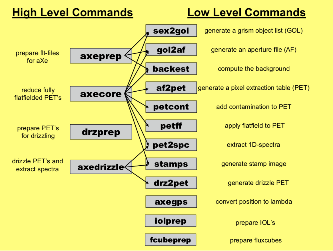
This figure is reproduced from the aXe User Manual.
aXedrizzle, for Processing G800L Data
The aXe/HSTaXe data reduction is based on the individual extraction of object beams on each flt.fits science image. ACS datasets usually consist of several images, with small position shifts or dithers between them. The aXedrizzle technique offers the possibility to combine the first order beams of each object extracted from a set of dithered G800L slitless spectra images, taken with the WFC and HRC.
The input for aXedrizzle consists of flat-fielded and wavelength-calibrated pixels extracted for all beams on each science image. For each beam, those pixels are stored as stamp images in multi-extension FITS files.
For each beam, aXe/HSTaXe computes transformation coefficients which are required to drizzle the single stamp images of each object onto a single deep, combined 2D spectral image. These transformation coefficients are computed such that the combined drizzled image resembles an ideal long slit spectrum with the dispersion direction parallel to the x-axis and cross-dispersion direction parallel to the y-axis. The wavelength scale and the pixel scale in the cross-dispersion direction can be set by the user with keyword settings in the aXe/HSTaXe configuration file.
If the set of slitless images to drizzle has a range of position angles, then caution is required in the use of aXedrizzle. Since the shape of the dispersing object acts as the "slit" for the spectrum, the object's orientation and length may differ for extended objects which are not circular. Naively combining the slitless spectra at different position angles with aXedrizzle will result in an output spectrum which suffers distortions—the resultant 1D extracted spectrum would be a poor representation of the real spectrum.
To extract the final 1D spectrum from the deep 2D spectral image, aXe/HSTaXe uses an (automatically created) adapted configuration file that takes into account the modified spectrum of the drizzled images (i.e., orthogonal wavelength and cross-dispersion, and the Å/pixel and arcsec/pixel scales).
Figure 5.10: Illustration of the aXedrizzle Process for One Object
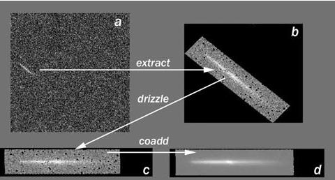
Panel (a) shows one individual grism image with an object marked. Panel (b) displays the stamp image for this object out of the grism image (a). Panel (c) shows the drizzled grism stamp image derived from (a), and the final co-added 2D spectrum for this object is given in panel (d).
Background Subtraction
aXe/hstaxe has two different strategies for removal of the sky background from the spectra.
The first strategy is to perform a global subtraction of a scaled "master sky" frame from each input spectrum image at the beginning of the reduction process. This removes the background signature from the images; the remaining signal can be assumed to originate only from the sources, and is extracted without further background correction in the aXe/hstaxe reduction. Master sky frames for the HRC and WFC G800L configurations are available for download from links given on the ACS Prism/Grism web page.
The second strategy is to make a local estimate of the sky background for each beam by interpolating between the adjacent pixels on either side of the beam. In this case, an individual sky estimate is made for every beam in each science image. This individual sky estimate is processed (flat-fielded, wavelength-calibrated) parallel to the original beam. Subtracting the 1D spectrum extracted from the sky estimate from the 1D spectrum derived from the original beam results finally in the pure object spectrum.
Output Products: Extracted Spectra
The primary output of aXe/HSTaXe is the file of extracted spectra (SPC). This is a multi-extension FITS binary table with as many table extensions as there are extracted beams. The beams are designated by an alphabetic postscript that correspond to the order defined by the configuration file. For example, the G800L WFC 1st order is BEAMA in the configuration file ACS.WFC*.conf. See the WFC3 G800L webpage for more information.
For instance, a first-order spectrum of an object designated as number 8 in an input Sextractor catalog, for WFC1 of the slitless image grism.fits, would be accessed as grism_5.SPC.fits[BEAM_8A]. That table contains 12 columns:wavelength; total, extracted, and background counts along with their associated errors; calibrated flux with its error and weight; a contamination flag. The header of the primary extension of the SPC table is a copy of the header of the frame from which the spectrum was extracted.
aXe/HSTaXe can also create, for each beam, a stamp image for the individual inspection of single beams. The stamp images of all beams extracted from a grism image are stored as a multi-extension FITS file with each extension containing the image of a single extracted beam. The stamp image of the first order spectrum of object number 8 from the above example would be stored as grism_5.STP.fits[BEAM_8A]. It is also possible to create stamp images for 2D drizzled grism images.
Other output products such as Pixel Extraction Tables, contamination maps, or Object Aperture Files are intermediate data products and their contents are not normally inspected.
Handling the aXe/HSTaXe Output
The output products from aXe/HSTaXe consist of ASCII files, FITS images, and FITS binary tables. The FITS binary tables containing wavelength, flux and flux uncertainties can be plotted as shown in Figure 5.11.
Figure 5.11: Example WFC G800L Extracted Spectrum
Tuning the Extraction Process
All aXe/HSTaXe tasks have several parameters which may be tuned in various ways to alter or improve the extraction. Please see the aXe User Manual for further details.
5.6.5 Accuracy of Slitless Spectra Wavelength and Flux Calibration
Wavelength Calibration
The dispersion solution was established by observing astronomical sources with known emission lines (e.g., for the WFC G800L and the HRC G800L, Wolf-Rayet stars were observed; see ACS ISR 2003-01, ACS ISR 2003-07, ACS ISR 2019-01. The field variation of the dispersion solution was mapped by observing the same star at different positions over the field. The internal accuracy of these dispersion solutions is good (see the ISR's for details) with an rms generally less than 0.2 pixels.
For a given object, the accuracy of the assigned wavelengths depends most sensitively on the accuracy of the zeropoint and the transfer of the zeropoint from the direct image to the slitless spectrum image. Provided that both direct and slitless images were taken with the same set of guide stars, systematic pointing offsets less than 0.2 pixels can be expected. For faint sources the error on the determination of the object centroid for the direct image will also contribute to wavelength error. Realistic zeropoint errors of up to 0.3 pixels are representative. For the highest wavelength accuracy it is advised to perform a number of pixel offsets of about ten percent of the field size for each of several direct and slitless image pairs and average the extracted spectra.
Flux Calibration
The sensitivity of the dispersers was established by observing a spectrophotometric standard star at several positions across the field. The sensitivity (aXe/HSTaXe uses a sensitivity tabulated in ergs/cm/cm/sec/Å per detected Å) was derived using data flat-fielded by the flat-field cube (see Section 5.6.2). In fact, the adequacy of the WFC flat field was established by comparing the detected counts in the standard star spectra at several positions across the field. These tests showed that the sensitivity at the peak of the WFC G800L varied by less than 5% across the whole field. However at the lower sensitivity edges of the spectra, to the blue (<5,800Å) and to the red (>10,000Å), the counts in the standards are low, and the errors in flux calibration approach 20%. In addition, small errors in wavelength assignment have a large effect in the blue and red where the sensitivity changes rapidly with wavelength. This often leads to strong upturns at the blue and red ends of extracted flux calibrated spectra, whose reality may be considered suspect. See ST-ECF ISR 2008-01.
1 Controls the automatic scheduling of image exposures for the purpose of spectra zero point determination of grism observations. By default, a single short image through a standard filter will be taken in conjunction with each Exposure Specification using the grism for external science observations.
2 (dispersion solutions have been derived for orders –3, –2, –1, 0, 1, 2 and 3 for the WFC G800L for example; see ACS ISR 2003-01)
3 This placeholder (dummy) flat corrects the gain offsets between the four WFC quadrants. For the HRC, which has only one amplifier, a single gain value is used. There is no gain correction for the SBC.