FUV Grating G140L
Description
G140L is a low-resolution grating (R ~ 2000) with wavelength coverage extending to 900 Å, and perhaps below. Its sensitivity at EUV wavelengths, marked in light blue in Figure 13.14, has not been calibrated. The grating has three central-wavelength settings: 800, 1105, and 1280 Å.
Special Considerations
The gap between Segments A and B spans 105 Å. When settings 800 or 1105 are used, the high voltage on Segment B must be lowered to avoid a dangerously high count rate from zero-order light. Wavelengths longer than 2150 Å may be contaminated by second-order light.
| Grating | Resolving Power R = λ/Δλ | Dispersion (mÅ pixel−1) | Plate Scale (milliarcsec pixel−1) | FP-POS Step (Å step−1) | |
|---|---|---|---|---|---|
| Disp. Axis | Cross-Disp. Axis | ||||
| G140L | 1,500–4,000 | 80.3 | 23.0 | 90 | 20.1 |
Figure 13.14: Wavelength Ranges for the G140L Grating.
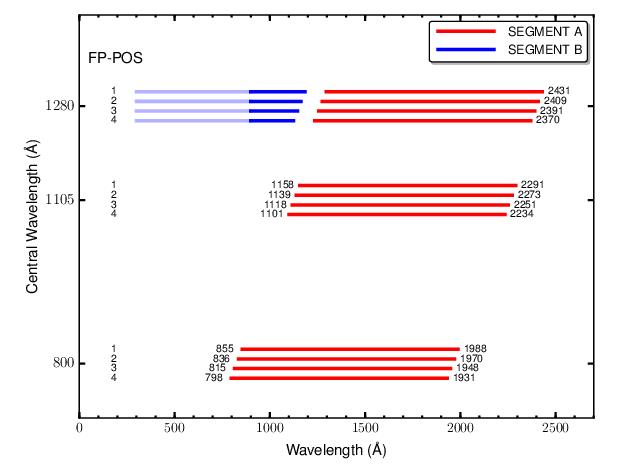
The COS sensitivity at EUV wavelengths (marked in light blue) is not known.
G140L Point-Source Sensitivity
Table 13.7: G140L Point-Source Sensitivity for PSA.
| Wavelength (Å) | Throughput | Sensitivity (counts pixel−1 sec−1 per erg cm−2 sec−1 Å−1) | Effective Area (cm2) |
|---|---|---|---|
914 | 1.907e−02 | 1.6e+12 | 1.82e+03 |
950 | 2.701e−04 | 1.5e+12 | 1.75e+03 |
1000 | 2.025e−04 | 1.3e+12 | 1.49e+03 |
1050 | 4.370e−04 | 1.1e+12 | 1.14e+03 |
1100 | 3.869e−02 | 8.6e+11 | 9.00e+02 |
1150 | 2.098e−02 | 6.6e+11 | 6.70e+02 |
1200 | 3.143e−02 | 5.0e+11 | 4 97e+02 |
1250 | 3.481e−02 | 4.2e+11 | 4.01e+02 |
1300 | 3.191e−02 | 3.6e+11 | 3.34e+02 |
| 1350 | 2.642e−02 | 2.7e+11 | 2.45e+02 |
| 1400 | 2.117e−02 | 5.4e+12 | 9.58e+02 |
| 1450 | 1.726e−02 | 4.5e+12 | 7.81e+02 |
| 1500 | 1.369e−02 | 3.7e+12 | 6.19e+02 |
| 1550 | 1.052e−02 | 2.9e+12 | 4.76e+02 |
| 1600 | 8.191e−03 | 2.4e+12 | 3.71e+02 |
| 1650 | 6.315e−03 | 1.9e+12 | 2.86e+02 |
| 1700 | 5.209e−03 | 1.6e+12 | 2.36e+02 |
| 1750 | 4.523e−03 | 1.4e+12 | 2.05e+02 |
| 1800 | 3.648e−03 | 1.2e+12 | 1.65e+02 |
| 1850 | 2.789e−03 | 9.3e+11 | 1.26e+02 |
| 1900 | 1.829e−03 | 6.3e+11 | 8.27e+01 |
| 1950 | 1.012e−03 | 3.6e+11 | 4.58e+01 |
| 2000 | 3.978e−04 | 1.4e+11 | 1.80e+01 |
| 2050 | 1.308e−04 | 4.9e+10 | 5.92e+00 |
| 2100 | 4.006e−05 | 1.5e+10 | 1.81e+00 |
| 2148 | 5.357e−06 | 2.1e+09 | 2.42e−01 |
Figure 13.15: G140L Point-Source Sensitivity for PSA and BOA.
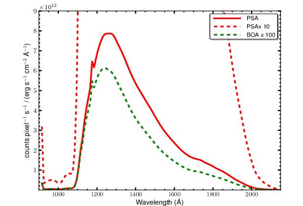
PSA × 10 is plotted to show sensitivity below 1100 Å.
G140L Signal-to-Noise Ratio
Figure 13.16: Point-Source Signal-to-Noise as a Function of STMAG for G140L.
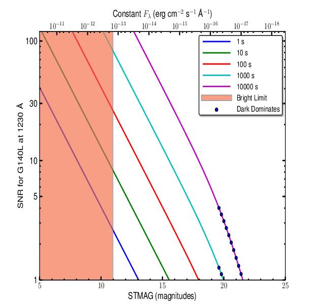
The top axis displays constant Fλ values corresponding to the STMAG units (V+STMAGλ) on the bottom axis. Recall that STMAG = 0 is equivalent to Fλ = 3.63E−9 erg cm−2 s−1 Å−1. Colors refer to exposure times in seconds. The edge of the shaded area corresponds to the bright-object screening limit. Use of the PSA is assumed.
-
COS Instrument Handbook
- Acknowledgments
- Chapter 1: An Introduction to COS
- Chapter 2: Proposal and Program Considerations
- Chapter 3: Description and Performance of the COS Optics
- Chapter 4: Description and Performance of the COS Detectors
-
Chapter 5: Spectroscopy with COS
- 5.1 The Capabilities of COS
- • 5.2 TIME-TAG vs. ACCUM Mode
- • 5.3 Valid Exposure Times
- • 5.4 Estimating the BUFFER-TIME in TIME-TAG Mode
- • 5.5 Spanning the Gap with Multiple CENWAVE Settings
- • 5.6 FUV Single-Segment Observations
- • 5.7 Internal Wavelength Calibration Exposures
- • 5.8 Fixed-Pattern Noise
- • 5.9 COS Spectroscopy of Extended Sources
- • 5.10 Wavelength Settings and Ranges
- • 5.11 Spectroscopy with Available-but-Unsupported Settings
- • 5.12 FUV Detector Lifetime Positions
- • 5.13 Spectroscopic Use of the Bright Object Aperture
- Chapter 6: Imaging with COS
- Chapter 7: Exposure-Time Calculator - ETC
-
Chapter 8: Target Acquisitions
- • 8.1 Introduction
- • 8.2 Target Acquisition Overview
- • 8.3 ACQ SEARCH Acquisition Mode
- • 8.4 ACQ IMAGE Acquisition Mode
- • 8.5 ACQ PEAKXD Acquisition Mode
- • 8.6 ACQ PEAKD Acquisition Mode
- • 8.7 Exposure Times
- • 8.8 Centering Accuracy and Data Quality
- • 8.9 Recommended Parameters for all COS TA Modes
- • 8.10 Special Cases
- Chapter 9: Scheduling Observations
-
Chapter 10: Bright-Object Protection
- • 10.1 Introduction
- • 10.2 Screening Limits
- • 10.3 Source V Magnitude Limits
- • 10.4 Tools for Bright-Object Screening
- • 10.5 Policies and Procedures
- • 10.6 On-Orbit Protection Procedures
- • 10.7 Bright Object Protection for Solar System Observations
- • 10.8 SNAP, TOO, and Unpredictable Sources Observations with COS
- • 10.9 Bright Object Protection for M Dwarfs
- Chapter 11: Data Products and Data Reduction
-
Chapter 12: The COS Calibration Program
- • 12.1 Introduction
- • 12.2 Ground Testing and Calibration
- • 12.3 SMOV4 Testing and Calibration
- • 12.4 COS Monitoring Programs
- • 12.5 Cycle 17 Calibration Program
- • 12.6 Cycle 18 Calibration Program
- • 12.7 Cycle 19 Calibration Program
- • 12.8 Cycle 20 Calibration Program
- • 12.9 Cycle 21 Calibration Program
- • 12.10 Cycle 22 Calibration Program
- • 12.11 Cycle 23 Calibration Program
- • 12.12 Cycle 24 Calibration Program
- • 12.13 Cycle 25 Calibration Program
- • 12.14 Cycle 26 Calibration Program
- • 12.15 Cycle 27 Calibration Program
- • 12.16 Cycle 28 Calibration Program
- • 12.17 Cycle 29 Calibration Program
- • 12.18 Cycle 30 Calibration Program
- • 12.19 Cycle 31 Calibration Program
- • 12.20 Cycle 32 Calibration Program
- • 12.21 Cycle 33 Calibration Program
- Chapter 13: COS Reference Material
- • Glossary