4.1 The FUV XDL Detector
4.1.1 XDL Properties
The COS FUV detector is a windowless cross delay line (XDL) device that is similar to the detectors used on the Far Ultraviolet Spectroscopic Explorer (FUSE). The XDL is a photon-counting micro-channel plate (MCP) detector with two independently operable segments (FUVA and FUVB). Each segment has an active area of 85 × 10 mm; they are placed end-to-end and separated by a 9-mm gap. When the locations of detected photons are digitized they are placed into a pair of arrays (one per detector), each 16,384 × 1,024 pixels, though the active area of the detector is considerably smaller. Individual pixels span 6 × 24 μm. The long dimension of the array is in the direction of dispersion; increasing pixel number (the detector’s x axis in user coordinates) corresponds to increasing wavelength. The XDL format is shown schematically in Figure 4.1. Detector parameters are listed in Table 1.2.
The FUV XDL is optimized for the 1150 to 1775 Å bandpass, with a cesium iodide photocathode on the front MCP. The front surfaces of the MCPs are curved with a radius of 826 mm to match the curvature of the focal plane. When photons strike the photocathode they produce photoelectrons that are multiplied by a stack of MCPs. The charge cloud that comes out of the MCP stack, several millimeters in diameter, lands on the delay-line anode. There is one anode for each detector segment, and each anode has separate traces for the dispersion (x) and cross-dispersion (y) axes. The location of an event on each axis is determined by measuring the relative arrival times of the collected charge pulse at each end of the delay-line anode for that axis. The results of this analog measurement are digitized to 14 bits in x and 10 bits in y. In TIME-TAG mode the total charge collected from the event, called the pulse height, is saved as a 5-bit number.
Figure 4.1: The FUV XDL Detector.
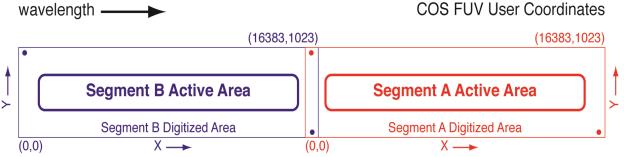
This diagram is drawn to scale, and the slight curvature at the corners is also present on the masks of the flight detectors. Wavelength increases in the direction of the increasing x coordinate. The red and blue dots show the approximate locations of the stim pulses (see 4.1.6 below) on each segment. The numbers in parentheses show the pixel coordinates at the corner of the segment’s digitized area; the two digitized areas overlap in the region of the inter-segment gap.
The XDLʹs quantum efficiency is improved by the presence of a series of wires, called the quantum-efficiency (QE) grid, placed above the detector (i.e., in the light path). These wires create shadows in the spectrum that are flagged and corrected by CalCOS during data reduction. The XDL also includes an ion-repeller grid that reduces the background rate by preventing low-energy thermal ions from entering the open-faced detector. It acts as a 95% transmission neutral-density filter.
4.1.2 XDL Spectrum Response
COS is considerably more sensitive than STIS and earlier-generation HST instruments at comparable spectral resolutions in the FUV. Effective areas for the COS FUV gratings are shown in Figure 5.1. The maximum count rates for the FUV detector are listed in Table 10.1. The time-dependent changes in the sensitivity of the COS FUV channel are discussed in Section 5.1.5.
4.1.3 XDL Dark Rate
The standard dark rate monitoring program is undertaken largely for the benefit of the exposure time calculator (ETC; see Section 7). Observations to ascertain dark rates are carried out through implementation of a variety of high voltages. If needed to support particular proposals, additional darks may be taken on a best effort basis if requested in Phase I files under Special Requirements. Users should note that darks are not guaranteed to have been taken on a concurrent timescale with science observations.
The XDL detector segments have extremely low intrinsic dark rates, on the order of 10–6 counts s-1 pixel-1; see Section 7.4.1. Background counts can also be caused be external events, such as proximity to the South Atlantic Anomaly (SAA). CalCOS estimates the dark rate by measuring the counts in an un-illuminated region on the detector and subtracting this from the spectrum during processing. Each segment has a distinct dark current that varies with time and may be correlated with the Solar Cycle (see Figure 4.2). The dark rates vary with time, so observers, particularly those with faint, background-limited targets, should consider how the changing dark rates may affect their orbital estimates. In particular, some exposures experience sharp increases in the dark rate over short periods of time. The COS spectroscopic ETC estimates the dark rate for a typical exposure and segment based on the value that encompasses 95% of all observations. For the ETC version 34.1.1, the dark rate assumed in science exposures is 3.15 × 10⁻⁶ counts s-1 pixel-1 for FUVA and 3.81 × 10⁻⁶ counts s-1 pixel-1 for FUVB. A webpage which monitors dark rates can be found at https://www.stsci.edu/hst/instrumentation/cos/performance/monitoring.
Figure 4.2: COS FUV Dark Rates and the Solar Cycle.
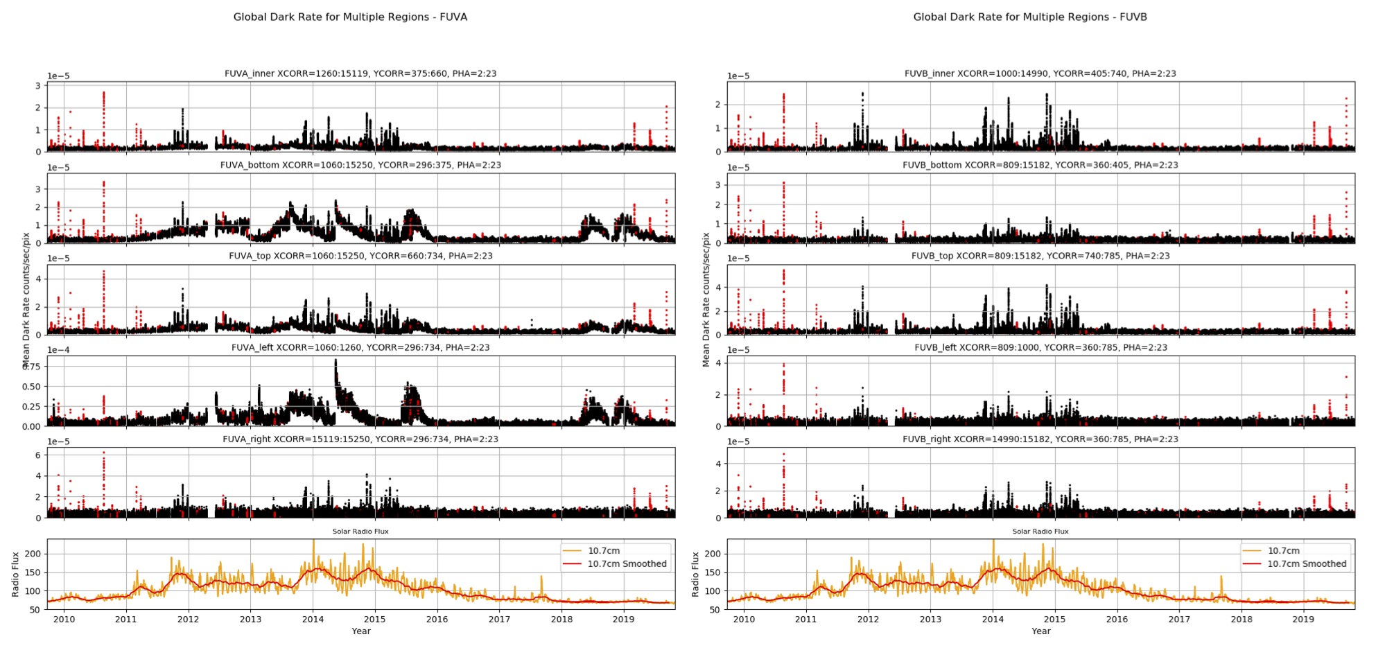
Left panel: COS/FUV dark rates on FUVA as a function of time for each of the different areas on the detector monitored. The top five panels show the measured dark rate in 25 s increments throughout every exposure. The red dots represent dark rates that were observed close to when HST was passing over the South Atlantic Anomaly. The bottom panel display the 10.7 cm solar radio emission, tracking the solar cycle. The orange curve shows the corresponding Solar Radio Emission, which is a proxy for stellar activity, a smoothed version of which is shown in red. The gap in data corresponds to the shutdown of COS due to a detector anomaly on April 30, 2012. Right panel: This is the same as the left panel, but for the COS FUVB detector. See COS ISR 2019-11 for further details on updates to COS FUV dark monitoring.
4.1.4 XDL Read-out Format
The FUV channel creates one spectral stripe on each detector segment for the science spectrum and another for the wavelength-calibration spectrum. The aperture not being used for science may also create a spectrum. If so, it will appear below the science spectrum if the PSA is being used, and above it if the target is in the BOA. Since the non-target aperture is usually observing blank sky, it will normally be visible only if airglow lines fall in the spectral range. Figure 4.3 shows an example of an FUV spectrum obtained on orbit with Segment B. The upper panel shows the two-dimensional image; the lower panel shows the extracted PSA spectrum. Note the difference in the x- and y-axis scales in the upper figure.
Although the gap between the two FUV detector segments prevents the recording of an uninterrupted spectrum, it can be made useful. For example, when the G140L grating is used with a central wavelength of 1280 Å, the bright Lyman-α airglow feature falls in the gap. For suggestions on spanning the gap, see Section 5.5.
Should a high count rate on one of the segments be a safety concern, the detector can be operated in single-segment mode, whereby the high voltage on one segment is lowered to a value that prevents it from detecting light. This adjustment is required for central wavelengths 800 Å and 1105 Å on G140L, since the zero-order light falling on Segment B in those modes is too bright.
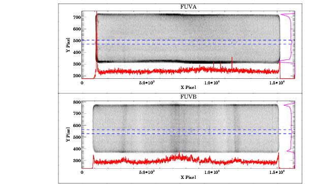
Figure 4.3: Example of a COS FUV Spectrum.
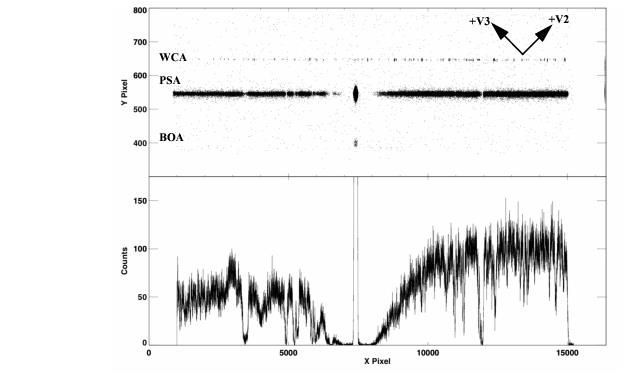
Upper panel: A stellar spectrum obtained with Segment B of the COS FUV detector using the G130M grating at a central wavelength of 1309 Å. (This configuration is not allowed by the COS 2025 policy.) The wavelength calibration (WCA) spectrum is on top, and the stellar spectrum (PSA) is below. Both the PSA and BOA are open to the sky when the COS shutter is open, so Lyman-α airglow through the BOA is also visible below the PSA. The HST +V2 and +V3 axes are over plotted. Note that the size of the active area of the MCP is smaller than the overall digitized area (16,384 × 1,024). Lower panel: the extracted stellar spectrum from the PSA.
4.1.5 Non-linear Photon Counting Effects (Dead Time)
The electronics that control the COS detectors have a finite response time t, called the dead time, that limits the rate at which photon events can be processed. If two photons arrive within time t, the second photon will not be processed. For the FUV channel three factors limit the detected count rate. The first is the Fast Event Counter (FEC) for each segment, which has a dead time of 300 ns. The FEC dead time matters only at count rates well above what is usable, introducing a 1% error at a count rate of 33,500 per segment per second.
The second factor is the time required to digitize a detected event. For a given true count rate C, the detected count rate D is:
| D=\frac{C}{1+C\times t}~, |
where t is the dead-time constant. For the COS FUV detector t = 7.4 μs, so the apparent count rate deviates from the true count rate by 1% when C = 1350 counts/s and by 10% when C = 15,000 counts/s. Note that, when the effect is near the 10% level, then the FUV detector is near its global count-rate screening limit (see Table 10.1), so non-linear effects are relatively small.
Finally, the Detector Interface Board (DIB) combines the count streams from the two FUV segments and writes them to a single data buffer. The DIB is limited to processing about 250,000 count/s in ACCUM mode and only 30,000 count/s in TIME-TAG mode (the highest rate allowed for TIME-TAG mode). The DIB interrogates the A and B segments alternately; because of this a count rate that is high in one segment, but not the other, could cause a loss of data from both segments. Tests have shown that the DIB is lossless up to a combined count rate for both segments of 20,000 count/s; the loss is 100 count/s at a rate of 40,000 count/s. Thus, this effect is less than 0.3% at the highest allowable rates. Furthermore, information in the engineering data characterizes this effect.
Corrections for dead-time effects are made in the CalCOS pipeline, but they are not included in the ETC, which will over-predict count rates for bright targets.
4.1.6 Stim Pulses
The signals from the XDL anodes are processed by Time-to-Digital Converters (TDCs). Each TDC contains a circuit that produces two alternating, periodic, negative-polarity pulses that are capacitively coupled to both ends of the delay-line anode. These stim pulses emulate counts located near the corners of the anode, beyond the active area of the detector. Stim pulses provide a means for CalCOS to correct the temperature-dependent shift and stretch of the image during an exposure, and they provide a first-order check on the dead-time correction. They are recorded in both TIME-TAG and ACCUM modes, and appear in the data files.
six stim-pulse rates are used: 0 (i.e., off), 2, 30, and 2000 Hz per segment. These rates, which are only approximate, are not user selectable. Exposures longer than 100 s will use the 2 Hz rate, those between 10 and 100 s use 30 Hz, and those shorter than 10 s use 2000 Hz.
4.1.7 Pulse-height Distributions
An ultraviolet photon incident on the front MCP of the XDL detector creates a shower of electrons, from which the detector electronics calculate the x and y coordinates and the total charge, or pulse height. The number of electrons created by each input photon, or "gain" of the MCPs, depends on the high voltage across the MCPs, the local properties of the MCPs at that location, and the high voltage across the plates. It is not a measure of the energy of the incident photon. A histogram of pulse heights for multiple events is called a pulse-height distribution (PHD).
The PHD from photon events on a particular region of the detector typically shows a peaked distribution, which can be characterized by the modal gain (the location of the peak) and its width. Background events, both internal to the detector and induced by cosmic rays, tend to have a falling exponential PHD, with most events having the lowest and highest pulse heights. On-board charge-threshold discriminators filter out very large and small pulses to reduce the background and improve the signal-to-noise ratio. In TIME-TAG mode the pulse height is recorded for each detected photon event. By rejecting outlier pulse-height events, CalCOS further reduces the background rate. In ACCUM mode only the integrated pulse-height distribution is recorded (Section 5.2.2), so pulse-height filtering is not possible.
Figure 4.4: Spectra Showing the Effects of Gain Sag on FUV Detector Segment B.
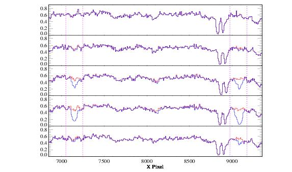
Spectra (G160M/1623/FP-POS=4) of a target observed five times over 19 months: from top to bottom, September 2009, June 2010, September 2010, January 2011, and May 2011. The blue curve includes only photon events with pulse heights in the range 4–30; the red curve includes pulse heights 2–30. The spectral features near pixels 7200 and 9011 are not astrophysical, but represent the effect of gain sag on regions of the detector illuminated by Lyman α in other observing modes. These features become more pronounced with time until March 2011, when the Segment B high voltage was raised.
Gain Sag
Prolonged exposure to light causes the number of electrons per incident photon to decrease, a phenomenon known as "gain sag." As a result, the peak of the PHD in each region of the detector shifts to lower values as the total (time-integrated) illumination of that region increases. As long as all pulse heights are above the minimum threshold imposed by the onboard electronics and CalCOS, there is no loss in sensitivity. However, if the gain drops low enough that the pulse heights of the photon events from the target fall below the threshold, these events are discarded and the apparent throughput decreases. The amount of gain sag increases with the total amount of previous illumination at that position on the detector, so gain sag appears first in regions of the detector that are illuminated by bright airglow lines, but eventually affects the entire spectrum. Figure 4.4 shows the effect of gain sag on Segment B of the COS FUV detector. These data were obtained using the grating setting G160M/1623/FP-POS=4 at LP1. A portion of the extracted spectrum from the same object taken at five different times is shown. The blue curve was constructed using only photon events with pulse heights in the range 4–30, while the red curve includes pulse heights of 2–30. The current pulse height limits used by the COS pipeline are 2–23. Two regions that suffer the most serious gain sag are marked: the region near pixel 7200 is illuminated by Lyman α when grating setting G130M/1309/FP-POS=3 is used, and the region near pixel 9100 is illuminated by Lyman α when the setting is G130M/1291/FP-POS=3. Initially, the pulse heights were well above either threshold, so the blue and red curves are indistinguishable. As time progressed, all of the pulse heights decreased. However, the two Lyman-α regions decreased faster, causing the blue spectra to exhibit spurious absorption features. This trend continued until the Segment B high voltage was raised in March 2011. The bottom plot shows that increasing the voltage has recovered most of the lost gain.
More details on the gain sag can be found in the COS Data Handbook and COS ISR 2011-05.
Detector Walk
As the pulse height of a photon event decreases, the detector electronics begin to systematically miscalculate its position. On the COS FUV detector this effect, called detector walk, occurs in both x and y, but is much larger in the y (cross-dispersion) direction. The shift is approximately 0.5 pixel per pulse-height bin, which means that the entire spectrum may be shifted by several pixels, and the regions with the lowest gain may be noticeably shifted relative to the rest of the spectrum (Figure 4.5). In July 2025, new reference files to be used by CalCOS for TIME-TAG data were delivered to improve the geometric distortion and walk corrections for the FUV detector (see COS ISR 2025-07). In addition, the walk is uncorrected in ACCUM mode, where no pulse-height information is available. The spectral extraction should remain unaffected, because the extraction regions are large enough to include the misplaced counts.
Figure 4.5: Y-Walk on the FUV Detector.
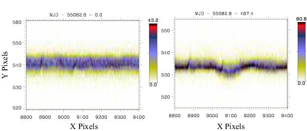
Two-dimensional spectra, uncorrected for walk, taken in September 2009 (left) and December 2010 (right). The entire spectrum has shifted down by several pixels due to gain sag and detector walk. A larger shift is seen in the region near X = 9100, where the gain sag is greater due to the geocoronal Lyman-α feature that falls there when the G130M/1291 when the FP-POS=3 setting is used.
Mitigation Strategies
A range of strategies have been used to minimize the effects of gain sag and detector walk on the science data. Several of these are modifications to CalCOS, which means that previously collected data can be improved by reprocessing. Others involve changes to the on-orbit settings, and thus only affect exposures taken after the changes are made.
CalCOS Changes
Pulse-Height Thresholding: At present, the lower pulse-height threshold used by CalCOS when processing TIME-TAG data has been decreased to near its minimum value (2). This ensures that as few events as possible are lost due to low gain, but it will have the effect of slightly increasing the detector background. We hope to eventually implement time- and position-dependent pulse-height thresholds in CalCOS.
Walk Correction: CalCOS applies a walk correction to TIME-TAG events. The pulse height and measured position of an event are used to apply a correction factor to its position. Although the walk correction is not time-dependent, it may be modified as we learn more about the walk properties of the detector.
Gain Sag Table: Low-gain pixels are flagged by CalCOS and excluded when combining spectra taken at multiple FP-POS positions.
Onboard Changes
Voltage Adjustments: In an effort to keep the MCP gain in the spectral regions within the range that gives acceptable position determination, while simultaneously minimizing gain sag, the high voltage on each segment has been adjusted numerous times since launch. The voltages used for a particular exposure can be found in the file headers, but the effects should be transparent to the user, since any effects on the data will be handled by CalCOS. More details on the high voltage changes are given in the COS Data Handbook.
Change in Lifetime Position: After years of collecting exposures—and tens of thousands of counts per pixel in the most exposed areas—the gain at certain areas on the MCPs drops so much that none of the techniques described above can return the detector to an acceptable level of performance. Once that occurs, the only way to obtain satisfactory data is to move the spectra to a new location on the detector, which can be accomplished by adjusting the position of the aperture and the pointing of HST. This moves the spectra to a pristine region on the detector, which defines a new lifetime position. COS has been operated at a total of eight lifetime positions. Because the optical path is slightly different for each lifetime position, the properties of the spectrograph are also slightly different. Thus, the resolving power, throughput, flat field, etc., may differ at different lifetime positions. A keyword in the header of the data files tells CalCOS which lifetime position was used, and reference files appropriate to that position are applied when processing the data.
Multiple LPs are in use simultaneously (see Section 5.12), with both the LP and high voltage chosen to optimize performance on the grating and central wavelength of each exposure. The position and voltage values are determined by STScI based on the performance of the detector, so they cannot be specified by general observers.
Details on associated new calibrations are reported in ISRs, the COS Data Handbook, and periodic STANs.
4.1.8 Spatial Variation of the Dark Rate
The dark rate varies spatially over the FUV detector. Figure 4.6 shows the sum of approximately 80,000 s of dark exposures taken over a five-month period in 2011. With the standard lower pulse-height threshold of 2, Segment A is relatively featureless away from the edges of the active area, except for a few small spots with a higher rate. Segment B shows several large regions with a slightly elevated rate; they are enhanced by less than a factor of two over the quieter regions.
For most TIME-TAG observations these features will have a negligible effect on the extracted spectra, because the variation is small and the overall rate is low (see Table 7.1). In ACCUM mode, where no lower pulse-height threshold is used, additional features appear. ACCUM mode is used only for bright targets, so these features should constitute a negligible fraction of the total counts.
Figure 4.6: FUV Detector Dark Features.
Summed dark exposures showing spatial variations on the detector. The approximate position of the G130M extraction window for the original lifetime position is marked in blue, and a sum of the dark counts in this extraction window as a function of x pixel is shown in red below the image. A sum as a function of y pixel is shown on the right side of the figure. Segment A is nearly featureless aside from a few small hot spots, while Segment B shows larger variations. Both segments show a slightly lower dark rate in the region where the most counts have fallen. This is due to gain sag. The data are binned by 8 pixels in each dimension for display purposes.
-
COS Instrument Handbook
- Acknowledgments
- Chapter 1: An Introduction to COS
- Chapter 2: Proposal and Program Considerations
- Chapter 3: Description and Performance of the COS Optics
- Chapter 4: Description and Performance of the COS Detectors
-
Chapter 5: Spectroscopy with COS
- 5.1 The Capabilities of COS
- • 5.2 TIME-TAG vs. ACCUM Mode
- • 5.3 Valid Exposure Times
- • 5.4 Estimating the BUFFER-TIME in TIME-TAG Mode
- • 5.5 Spanning the Gap with Multiple CENWAVE Settings
- • 5.6 FUV Single-Segment Observations
- • 5.7 Internal Wavelength Calibration Exposures
- • 5.8 Fixed-Pattern Noise
- • 5.9 COS Spectroscopy of Extended Sources
- • 5.10 Wavelength Settings and Ranges
- • 5.11 Spectroscopy with Available-but-Unsupported Settings
- • 5.12 FUV Detector Lifetime Positions
- • 5.13 Spectroscopic Use of the Bright Object Aperture
- Chapter 6: Imaging with COS
- Chapter 7: Exposure-Time Calculator - ETC
-
Chapter 8: Target Acquisitions
- • 8.1 Introduction
- • 8.2 Target Acquisition Overview
- • 8.3 ACQ SEARCH Acquisition Mode
- • 8.4 ACQ IMAGE Acquisition Mode
- • 8.5 ACQ PEAKXD Acquisition Mode
- • 8.6 ACQ PEAKD Acquisition Mode
- • 8.7 Exposure Times
- • 8.8 Centering Accuracy and Data Quality
- • 8.9 Recommended Parameters for all COS TA Modes
- • 8.10 Special Cases
- Chapter 9: Scheduling Observations
-
Chapter 10: Bright-Object Protection
- • 10.1 Introduction
- • 10.2 Screening Limits
- • 10.3 Source V Magnitude Limits
- • 10.4 Tools for Bright-Object Screening
- • 10.5 Policies and Procedures
- • 10.6 On-Orbit Protection Procedures
- • 10.7 Bright Object Protection for Solar System Observations
- • 10.8 SNAP, TOO, and Unpredictable Sources Observations with COS
- • 10.9 Bright Object Protection for M Dwarfs
- Chapter 11: Data Products and Data Reduction
-
Chapter 12: The COS Calibration Program
- • 12.1 Introduction
- • 12.2 Ground Testing and Calibration
- • 12.3 SMOV4 Testing and Calibration
- • 12.4 COS Monitoring Programs
- • 12.5 Cycle 17 Calibration Program
- • 12.6 Cycle 18 Calibration Program
- • 12.7 Cycle 19 Calibration Program
- • 12.8 Cycle 20 Calibration Program
- • 12.9 Cycle 21 Calibration Program
- • 12.10 Cycle 22 Calibration Program
- • 12.11 Cycle 23 Calibration Program
- • 12.12 Cycle 24 Calibration Program
- • 12.13 Cycle 25 Calibration Program
- • 12.14 Cycle 26 Calibration Program
- • 12.15 Cycle 27 Calibration Program
- • 12.16 Cycle 28 Calibration Program
- • 12.17 Cycle 29 Calibration Program
- • 12.18 Cycle 30 Calibration Program
- • 12.19 Cycle 31 Calibration Program
- • 12.20 Cycle 32 Calibration Program
- • 12.21 Cycle 33 Calibration Program
- Chapter 13: COS Reference Material
- • Glossary