7.5 Extinction Correction
Extinction can dramatically reduce the observed intensity of your source, particularly in the ultraviolet. Figure 7.3 shows Aλ/AV values applicable to our Galaxy, taken from Cardelli, Clayton, & Mathis (1989, ApJ, 345, 245) assuming RV = 3.1. This corresponds to the Milky Way Diffuse (Rv = 3.1) selection of the ETC.
Extinction curves have a strong metallicity dependence, particularly at ultraviolet wavelengths. Sample extinction curves are presented in Gordon et al. [2003, ApJ, 594, 279 (LMC Average, LMC 30 Dor Shell, and SMC Bar)], Calzetti et al. [2000, ApJ, 533, 682 (starburst galaxies)], and references therein. At lower metallicities, the 2200 Å bump that is so prominent in the Galactic extinction curve disappears, and Aλ/E(B – V) increases at shorter UV wavelengths.
The ETC allows the user to select among a variety of extinction curves and to apply the extinction correction either before or after the input spectrum is normalized. Be aware that not all extinction laws in the ETC extend below 1200 Å, which may cause incorrect calculations for the 1222, 1055, and 1096 Å central wavelengths.
Figure 7.3: Extinction in Magnitude as a Function of Wavelength.
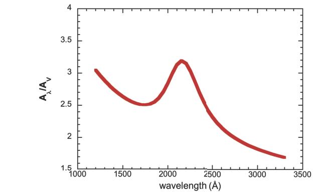
The Galactic extinction model of Cardelli et al. (1989), computed for RV = 3.1.
-
COS Instrument Handbook
- Acknowledgments
- Chapter 1: An Introduction to COS
- Chapter 2: Proposal and Program Considerations
- Chapter 3: Description and Performance of the COS Optics
- Chapter 4: Description and Performance of the COS Detectors
-
Chapter 5: Spectroscopy with COS
- 5.1 The Capabilities of COS
- • 5.2 TIME-TAG vs. ACCUM Mode
- • 5.3 Valid Exposure Times
- • 5.4 Estimating the BUFFER-TIME in TIME-TAG Mode
- • 5.5 Spanning the Gap with Multiple CENWAVE Settings
- • 5.6 FUV Single-Segment Observations
- • 5.7 Internal Wavelength Calibration Exposures
- • 5.8 Fixed-Pattern Noise
- • 5.9 COS Spectroscopy of Extended Sources
- • 5.10 Wavelength Settings and Ranges
- • 5.11 Spectroscopy with Available-but-Unsupported Settings
- • 5.12 FUV Detector Lifetime Positions
- • 5.13 Spectroscopic Use of the Bright Object Aperture
- Chapter 6: Imaging with COS
- Chapter 7: Exposure-Time Calculator - ETC
-
Chapter 8: Target Acquisitions
- • 8.1 Introduction
- • 8.2 Target Acquisition Overview
- • 8.3 ACQ SEARCH Acquisition Mode
- • 8.4 ACQ IMAGE Acquisition Mode
- • 8.5 ACQ PEAKXD Acquisition Mode
- • 8.6 ACQ PEAKD Acquisition Mode
- • 8.7 Exposure Times
- • 8.8 Centering Accuracy and Data Quality
- • 8.9 Recommended Parameters for all COS TA Modes
- • 8.10 Special Cases
- Chapter 9: Scheduling Observations
-
Chapter 10: Bright-Object Protection
- • 10.1 Introduction
- • 10.2 Screening Limits
- • 10.3 Source V Magnitude Limits
- • 10.4 Tools for Bright-Object Screening
- • 10.5 Policies and Procedures
- • 10.6 On-Orbit Protection Procedures
- • 10.7 Bright Object Protection for Solar System Observations
- • 10.8 SNAP, TOO, and Unpredictable Sources Observations with COS
- • 10.9 Bright Object Protection for M Dwarfs
- Chapter 11: Data Products and Data Reduction
-
Chapter 12: The COS Calibration Program
- • 12.1 Introduction
- • 12.2 Ground Testing and Calibration
- • 12.3 SMOV4 Testing and Calibration
- • 12.4 COS Monitoring Programs
- • 12.5 Cycle 17 Calibration Program
- • 12.6 Cycle 18 Calibration Program
- • 12.7 Cycle 19 Calibration Program
- • 12.8 Cycle 20 Calibration Program
- • 12.9 Cycle 21 Calibration Program
- • 12.10 Cycle 22 Calibration Program
- • 12.11 Cycle 23 Calibration Program
- • 12.12 Cycle 24 Calibration Program
- • 12.13 Cycle 25 Calibration Program
- • 12.14 Cycle 26 Calibration Program
- • 12.15 Cycle 27 Calibration Program
- • 12.16 Cycle 28 Calibration Program
- • 12.17 Cycle 29 Calibration Program
- • 12.18 Cycle 30 Calibration Program
- • 12.19 Cycle 31 Calibration Program
- • 12.20 Cycle 32 Calibration Program
- • 12.21 Cycle 33 Calibration Program
- Chapter 13: COS Reference Material
- • Glossary