3.3 The COS Line-Spread Function
The COS optics correct for the spherical aberration of the HST primary mirror, but not for the mid-frequency wavefront errors (MFWFEs) due to zonal (polishing) irregularities in the HST primary and secondary mirrors. As a result, the COS spectroscopic line-spread function (LSF) has extended wings and a core that is slightly broader and shallower than a Gaussian. The extended wings of its LSF limit the ability of COS to detect faint, narrow spectral features. The effect is greater at short wavelengths, and it may have consequences for some COS FUV science. The most severely impacted programs are likely to be those that:
- rely on models of the shapes of narrow lines,
- search for very weak lines,
- aim to measure line strengths in complex spectra with overlapping, or nearly overlapping, lines, or
- require precise estimates of residual intensity in very strong or saturated lines.
Modeled line spread functions and cross-dispersion spread functions are available for all cenwaves and LPs at https://www.stsci.edu/hst/instrumentation/cos/performance/spectral-resolution.
3.3.1 Non-Gaussianity of the COS LSF
Initial results from an analysis of the on-orbit COS LSF at the original lifetime position are reported by Ghavamian et al. (2009) in COS ISR 2009-01. They find that model LSFs incorporating HST MFWFEs are required to reproduce the absorption features observed in stellar spectra obtained with COS. Figure 3.6 shows model LSFs computed for grating G130M at 1309 Å. The dashed line represents a model incorporating the spherical aberration of the HST OTA. It is well-fit by a Gaussian with FWHM = 6.5 pixels. The solid black line represents a model that includes the MFWFEs at the original lifetime position, while the solid colored lines represent models that include the MFWFEs at subsequent lifetime positions. The model at the original lifetime position has a FWHM of 7.9 pixels, slightly larger than that of the dashed curve, and broad non-Gaussian wings. The models at subsequent lifetime positions have similar FWHM. The non-Gaussian wings can hinder the detection of closely-spaced narrow spectral features. Model LSFs for all of the COS gratings at the original and subsequent lifetime positions are available on the COS website.
Figure 3.6: Model Line-Spread Functions for the COS FUV Channel.
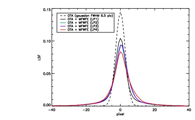
Model LSFs for G130M at 1309 Å normalized to a sum of unity. The dashed line represents a model LSF that incorporates the spherical aberration of the OTA. It is well fit by a Gaussian with FWHM = 6.5 pixels. The solid black line represents a model that also includes the HST mid-frequency wavefront errors at the original lifetime position. The solid colored lines represent models that include the HST mid-frequency wavefront errors at subsequent lifetime positions. These LSFs show a larger FWHM and broad non-Gaussian wings.
3.3.2 Quantifying the Resolution
When a substantial fraction of the power in an LSF is transferred to its extended wings traditional measures of resolution, such as the FWHM of the line core, can be misleading. For example, an observer assuming that the resolving power R = 16,000 at 1200 Å quoted for the G130M grating represents the FWHM of a Gaussian would mistakenly conclude that COS can resolve two closely-spaced narrow absorption features, when in fact it may not be able to. Nevertheless, the FWHM is a convenient measure, and we use it to describe the COS gratings in tables throughout this handbook. When using these tables keep in mind that the quoted resolving power R is computed from the empirically determined FWHM of the line core, and careful modeling may be needed to determine the feasibility of a particular observation or to analyze its result.
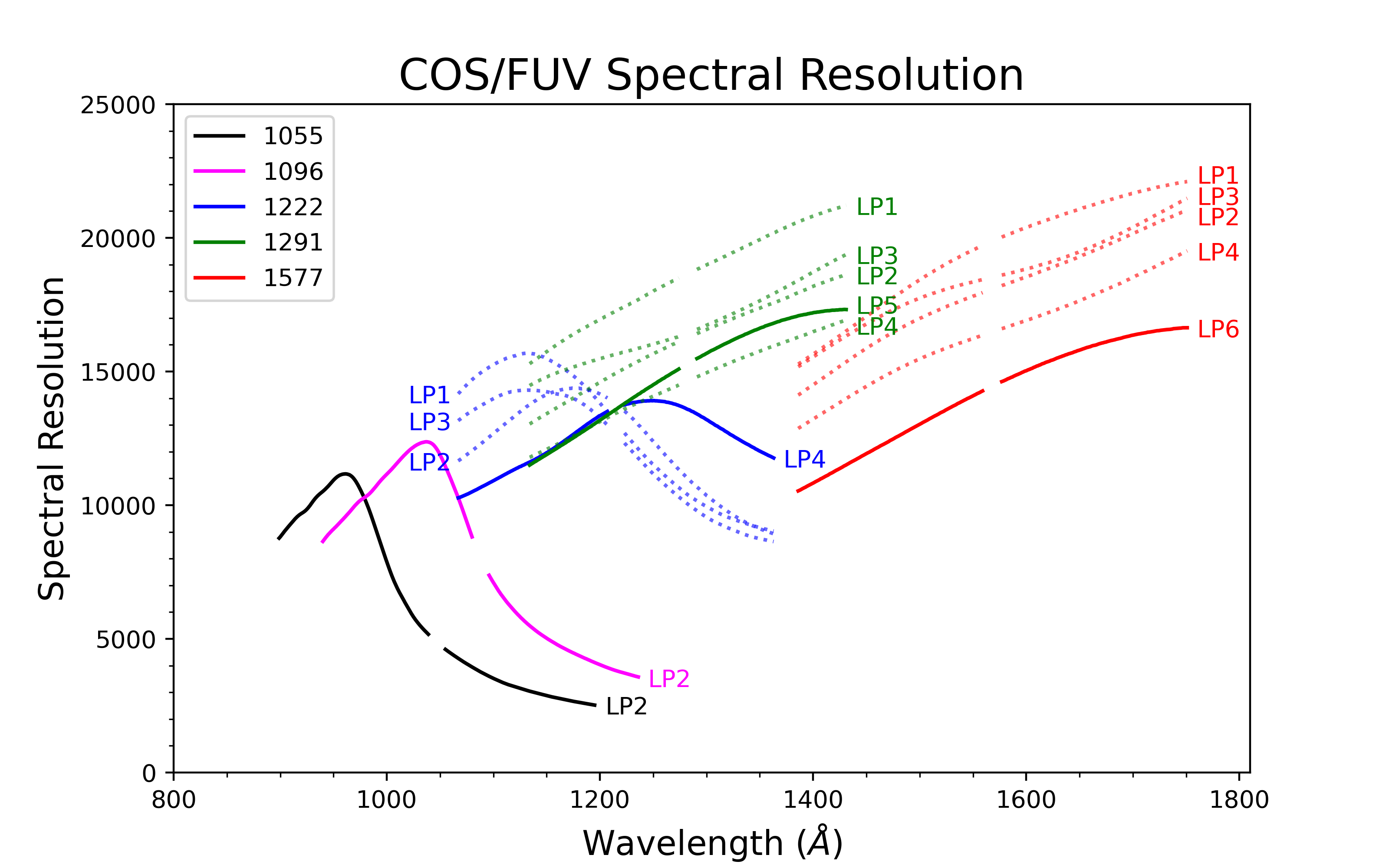
Figure 3.7 shows the resolving power of selected cenwaves.
Figure 3.7: Resolving Power of FUV Gratings at select cenwaves, and for all Lifetime Positions (LPs). Solid lines show the current default LP for each cenwave.
3.3.3 Impact on Equivalent Width Measurements
The broad core and extended wings of the COS LSF increase the limiting equivalent width for absorption features in COS spectra. Figure 3.8 shows the limiting equivalent widths as a function of wavelength for a 3σ FUV detection of absorption features at S/N = 10 per pixel at lifetime position 4. A series of Gaussian spectral features with nominal Doppler parameters of b = 0, 10, 25, 50, and 100 km/s have been convolved with both a Gaussian instrumental LSF and the modeled on-orbit COS LSF for the G130M and G160M gratings. The results are similar for the NUV gratings, although the effect of the MFWFEs is more moderate for the long-wavelength G285M grating.
Figure 3.8: Limiting Equivalent Width of FUV Medium-Resolution Gratings.
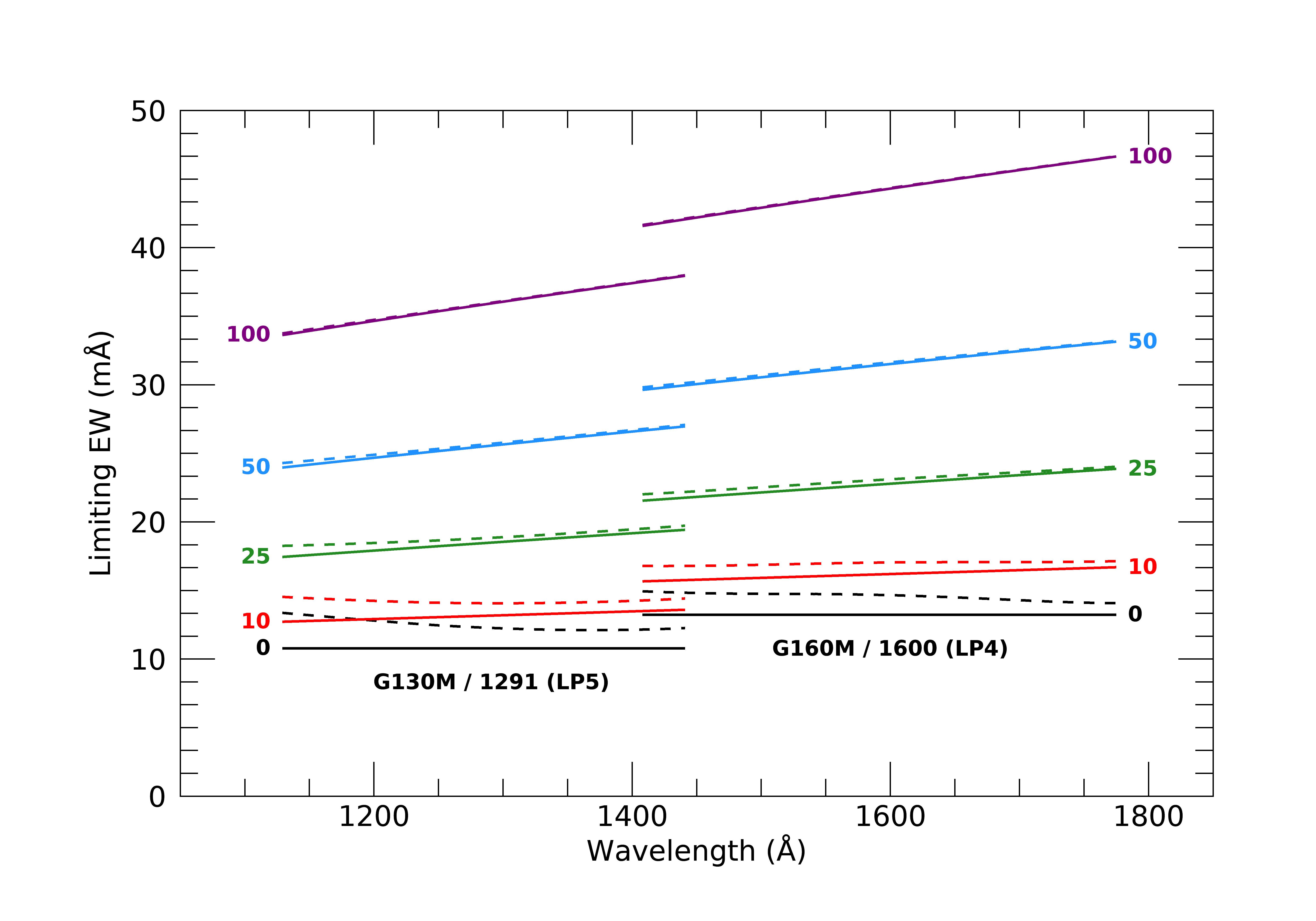
Limiting equivalent width as a function of wavelength for 3σ detections of absorption features at a S/N of 10 per pixel at lifetime position 5 (G130M/1291) and lifetime position 4 (G160M/1600). Dashed lines represent the full on-orbit LSFs including MFWFEs. Solid lines represent Gaussian LSFs without MFWFEs. The colors correspond to features with intrinsic Doppler parameters b = 0 km s-1 (black), 10 km s-1 (red), 25 km s-1 (green), 50 km s-1 (blue) and 100 km s-1 (purple).
3.3.4 Extended Wings of the COS LSF
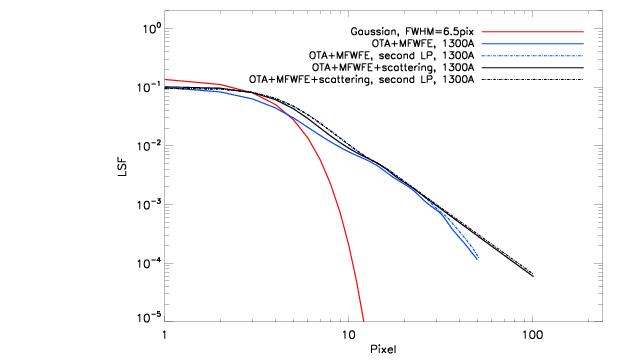
The LSF models of Ghavamian et al. (2009) successfully characterize the basic profile and integrated properties of narrow spectral features in COS spectra. However, scientific investigations that depend on characterizing the depth of saturated or nearly-saturated absorption features may require a more careful treatment of the light scattered into the wings of the LSF. To address this concern, Kriss (2011) in COS ISR 2011-01 has developed empirical LSF models for the G130M and G160M gratings. These models differ in two ways from the preliminary models discussed above. First, while the preliminary models extend only ±50 pixels from the line center, the new models extend ±100 pixels, which is the full width of the geocoronal Lyman-α line. Second, the new models include scattering due to the micro-roughness of the surface of the primary mirror, an effect that transfers an additional 3% of the light from the center of the line into its extended wings (Figure 3.9). For details, see COS ISR 2011-01. The LSF models computed by Ghavamian et al. (2009) and predicted LSFs for the lifetime positions are available on the COS website.
Figure 3.9: Comparison of LSF Models for Medium-Resolution FUV Gratings.
3.3.5 Enclosed Energy of COS LSF
Figure 3.10 shows the fraction of enclosed energy within the LSF, measured from the center of the profile, for both the FUV and NUV channels. The differences between the modeled on-orbit LSFs (MFWFEs included) and the Gaussian LSFs without MFWFEs are apparent in both spectroscopic channels. Though inclusion of the MFWFEs at longer NUV wavelengths widens the FWHM of the on-orbit LSF models only slightly, the wider wings decrease noticeably the spectral purity and the contrast level of the observed spectra.
Figure 3.10: Enclosed Energy Fraction of the COS Line-Spread Function.
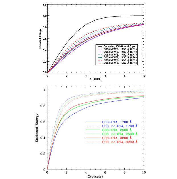
The enclosed energy fraction of the COS LSF for an unresolved spectral feature as measured from the center of the profile (collapsed along the cross-dispersion direction). The top panel shows a Gaussian with FWHM = 6.5 px and FUV model profiles. The 1150 Å data (purple) use the G130M grating, while the 1450 Å (teal) and 1750 Å (red) data use the G160M grating. The dashed lines indicate results for the original lifetime position, while the solid lines indicate data for the fourth lifetime position. In the bottom panel, NUV model profiles with and without the effects of the OTA MFWFEs are shown (Ghavamian et al. 2009). The 1700 Å data (blue) use the G185M grating, the 2500 Å data (green) use the G225M grating, and the 3200 Å data (red) use the G285M grating.
| Enclosed Energy Fraction | Wavelength (Å) | ||||||
|---|---|---|---|---|---|---|---|
| 1150 | 1200 | 1250 | 1300 | 1350 | 1400 | 1450 | |
0.90 | 14.9/15.2 | 15.0/15.1 | 15.0/14.9 | 14.9/15.2 | 14.8/14.5 | 14.7/14.2 | 14.4/14.7 |
0.95 | 24.3/24.7 | 24.4/24.6 | 24.4/24.3 | 24.5/24.8 | 24.4/23.9 | 24.3/23.3 | 23.8/24.3 |
0.99 | 58.1/58.6 | 58.3/58.4 | 58.3/58.0 | 58.4/58.7 | 58.3/57.5 | 58.2/57.1 | 57.5/58.1 |
Table 3.3: Distance from Line Center (in Pixels) versus Enclosed Energy Fraction and Wavelength for the G160M Grating.2
| Enclosed Energy Fraction | Wavelength (Å) | ||||||
|---|---|---|---|---|---|---|---|
| 1450 | 1500 | 1550 | 1600 | 1650 | 1700 | 1750 | |
0.90 | 14.7/14.4 | 14.6/14.9 | 14.4/14.2 | 14.2/14.0 | 14.0/13.8 | 13.6/13.7 | 13.2/13.2 |
0.95 | 24.5/24.0 | 24.3/24.7 | 24.0/23.8 | 23.8/23.7 | 23.5/23.4 | 23.1/23.1 | 22.6/22.8 |
0.99 | 58.3/57.6 | 58.1/58.7 | 57.8/57.4 | 57.4/57.1 | 57.0/56.8 | 56.3/56.4 | 55.6/55.9 |
Table 3.4: Distance from Line Center (in Pixels) versus Enclosed Energy Fraction and Wavelength for the G140L Grating.3
| Enclosed Energy Fraction | Wavelength (Å) | |||||||||||
|---|---|---|---|---|---|---|---|---|---|---|---|---|
| 1250 | 1300 | 1350 | 1400 | 1450 | 1500 | 1550 | 1600 | 1650 | 1700 | 1750 | 1800 | |
0.90 | 12.1 | 12.1 | 12.1 | 12.1 | 12.1 | 12.1 | 12.0 | 11.9 | 11.8 | 11.7 | 11.6 | 11.4 |
0.95 | 17.9 | 18.1 | 18.2 | 18.4 | 18.5 | 18.6 | 18.7 | 18.7 | 18.7 | 18.7 | 18.7 | 18.7 |
0.99 | 30.5 | 30.7 | 31.0 | 31.3 | 31.6 | 31.9 | 32.1 | 32.4 | 32.6 | 32.9 | 33.2 | 33.3 |
Table 3.2, Table 3.3, and Table 3.4 present the enclosed-energy fractions for gratings G130M, G160M, and G140L respectively. The distances reported in the tables are half-widths. The G130M and G160M data include the effects of scattering and are for both the original and the second lifetime position. Values for subsequent lifetime positions are not expected to differ appreciably. The G140L data are taken from Ghavamian et al. (2009) and are for the original lifetime position. The G140L data do not include the effects of micro-roughness. Please see the COS website for updated cenwave-dependent tabulations of the LSFs at all lifetime positions.
1The values in each cell are from the original lifetime position/second lifetime position.
2The values in each cell are from the original lifetime position/second lifetime position.
3The values in each cell are from the original lifetime position.
-
COS Instrument Handbook
- Acknowledgments
- Chapter 1: An Introduction to COS
- Chapter 2: Proposal and Program Considerations
- Chapter 3: Description and Performance of the COS Optics
- Chapter 4: Description and Performance of the COS Detectors
-
Chapter 5: Spectroscopy with COS
- 5.1 The Capabilities of COS
- • 5.2 TIME-TAG vs. ACCUM Mode
- • 5.3 Valid Exposure Times
- • 5.4 Estimating the BUFFER-TIME in TIME-TAG Mode
- • 5.5 Spanning the Gap with Multiple CENWAVE Settings
- • 5.6 FUV Single-Segment Observations
- • 5.7 Internal Wavelength Calibration Exposures
- • 5.8 Fixed-Pattern Noise
- • 5.9 COS Spectroscopy of Extended Sources
- • 5.10 Wavelength Settings and Ranges
- • 5.11 Spectroscopy with Available-but-Unsupported Settings
- • 5.12 FUV Detector Lifetime Positions
- • 5.13 Spectroscopic Use of the Bright Object Aperture
- Chapter 6: Imaging with COS
- Chapter 7: Exposure-Time Calculator - ETC
-
Chapter 8: Target Acquisitions
- • 8.1 Introduction
- • 8.2 Target Acquisition Overview
- • 8.3 ACQ SEARCH Acquisition Mode
- • 8.4 ACQ IMAGE Acquisition Mode
- • 8.5 ACQ PEAKXD Acquisition Mode
- • 8.6 ACQ PEAKD Acquisition Mode
- • 8.7 Exposure Times
- • 8.8 Centering Accuracy and Data Quality
- • 8.9 Recommended Parameters for all COS TA Modes
- • 8.10 Special Cases
- Chapter 9: Scheduling Observations
-
Chapter 10: Bright-Object Protection
- • 10.1 Introduction
- • 10.2 Screening Limits
- • 10.3 Source V Magnitude Limits
- • 10.4 Tools for Bright-Object Screening
- • 10.5 Policies and Procedures
- • 10.6 On-Orbit Protection Procedures
- • 10.7 Bright Object Protection for Solar System Observations
- • 10.8 SNAP, TOO, and Unpredictable Sources Observations with COS
- • 10.9 Bright Object Protection for M Dwarfs
- Chapter 11: Data Products and Data Reduction
-
Chapter 12: The COS Calibration Program
- • 12.1 Introduction
- • 12.2 Ground Testing and Calibration
- • 12.3 SMOV4 Testing and Calibration
- • 12.4 COS Monitoring Programs
- • 12.5 Cycle 17 Calibration Program
- • 12.6 Cycle 18 Calibration Program
- • 12.7 Cycle 19 Calibration Program
- • 12.8 Cycle 20 Calibration Program
- • 12.9 Cycle 21 Calibration Program
- • 12.10 Cycle 22 Calibration Program
- • 12.11 Cycle 23 Calibration Program
- • 12.12 Cycle 24 Calibration Program
- • 12.13 Cycle 25 Calibration Program
- • 12.14 Cycle 26 Calibration Program
- • 12.15 Cycle 27 Calibration Program
- • 12.16 Cycle 28 Calibration Program
- • 12.17 Cycle 29 Calibration Program
- • 12.18 Cycle 30 Calibration Program
- • 12.19 Cycle 31 Calibration Program
- • 12.20 Cycle 32 Calibration Program
- • 12.21 Cycle 33 Calibration Program
- Chapter 13: COS Reference Material
- • Glossary