7.2 The CCD
7.2.1 Detector Properties
The STIS CCD is a low-noise device capable of high sensitivity in the visible and the NUV. It is a thinned, backside-illuminated device manufactured by Scientific Imaging Technologies (SITe). In order to provide NUV imaging performance, the CCD was backside-treated and coated with a wide-band anti-reflectance coating. The process produces acceptable NUV quantum efficiency (QE) without compromising the high QE of the visible bandpass. The CCD camera design incorporates a warm dewar window, designed to prevent buildup of contaminants on the window, which were found to cause a loss of UV throughput for the WFPC2 CCDs. A summary of the STIS CCD performance is given in Table 7.1. Read noise and dark current values are based on data taken in Cycle 30. See the STIS website for further updates.
Table 7.1: CCD Detector Performance Characteristics.
Characteristic | CCD Performance |
Architecture | Thinned, backside illuminated |
Wavelength range | 1640–10,300 Å |
Pixel format | 1024 × 1024 illuminated pixels |
Field of view | 52 × 52 arcseconds2 |
Pixel size | 21 × 21 micrometers2 |
Pixel plate scale | 0.05078 arcseconds |
Quantum efficiency | ∼20% @ 3000 Å |
Dark count rate | 0.029 e−/s/ pix (but varies with detector temperature and Y-position) |
Read noise (Amp D) | 6.2 e− rms at |
Full well | 128,000 e− over the inner portion of the detector |
Saturation limit | 33,000 e− at |
7.2.2 Effects of the Change to STIS Side-2 Electronics on CCD Performance
In May 2001, the primary Side-1 electronics on STIS failed. Operations were subsequently resumed using the backup Side-2 electronics. CCD observations have been affected in two ways.
First, the Side-2 electronics do not have a working CCD temperature controller, and the detector can no longer be held at a fixed temperature. As a result, the CCD dark current now fluctuates with the detector temperature. Fortunately, the dark current variation correlates with the CCD housing temperature. The dark current scales with housing temperature at a rate between 5% and 10%/°C, depending upon the individual pixel and when the exposure was taken in the lifetime of STIS. This is approximated by a 7%/°C correction. Further details are given in STIS ISR 2001-03, STIS ISR 2018-05, and references therein. All reference file dark images prepared for use with STIS/CCD data taken during Side-2 operations are now scaled to a standard housing temperature of 18°C before being delivered. Before subtraction of the appropriate dark file from Side-2 CCD data, the calstis package rescales the dark using the CCD housing temperature value in the OCCDHTAV keyword which is found in the extension header of each sub-exposure.
The second change is an increase in the read noise by about 1 electron when CCDGAIN=1 and by 0.2 electrons when CCDGAIN=4. This extra read noise appears in the form of coherent pattern noise, and under some circumstances it may be possible to reduce this noise by using Fourier filtering techniques. A discussion of this can be found in STIS ISR 2001-05 and the astronomical community has produced other methods of subtracting out this noise (see the conference proceeding from the HST Calibration Workshop on the IDL code Autofilet.pro). Users who wish to have access to the Autofilet.pro code should contact the HST Help Desk.
7.2.3 STIS CCD Performance After Repair During SM4
The repair made during SM4 restored the Side-2 electronics to operation; the failure that had affected Side-1 electronics was not accessible, and the Side-1 electronics remain inoperative. As a result, the changes to CCD operations introduced by the switch to the Side-2 electronics, including both the inability to actively control the CCD chip temperature and the extra coherent pattern noise discussed above, continue to affect STIS operations after the repair. For additional information please see STIS ISR 2009-02.
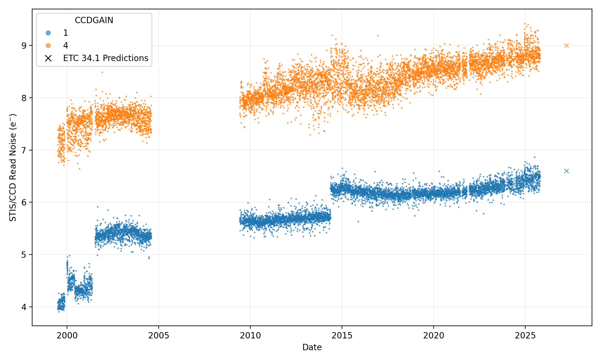
Changes in CCD Read Noise
The coherent pattern noise appears to be unchanged in its amplitude and behavior, however, the overall read noise of the STIS CCD has increased after the repair. During the period of Side-2 operations, the mean read noise measured using the default readout amplifier with CCDGAIN=1 was 5.44 electrons; in the months after SM4 and during Cycle 17 calibrations the mean was 5.62 electrons. For CCDGAIN=4, the read noise increased from 7.6 electrons to 8.0 electrons. Similar increases in read noise were seen in the three other STIS CCD amplifiers.
A further increase in the Amp D read noise was seen on May 15, 2014, as shown in Figure 7.1. Shortly after this date, the CCDGAIN=1 read noise was 6.2 electrons, and that for CCDGAIN=4 was 8.5 electrons. (Amps A and C appear to have been unaffected at this time.) This increase is thought to have been caused by radiation damage early in the Amp D signal chain electronics. In September of 2016, Amp C showed an increase by ~7% and has remained steady at this new read noise value. Additional increases of this type are possible, and the read noise is monitored on a regular basis. Amp D continues to show the lowest read noise among the four amplifiers; it remains the default amplifier and is used for all GO science exposures. Figure 7.1 shows the CCD read noise for Amp D across both pre- and post-SM4. Projected read noise values for the Cycle 34 ETC are included for both the CCDGAIN=1 and CCDGAIN=4 settings, which are 6.6 and 9.0 electrons, respectively.
CCDGAIN=1 and CCDGAIN=4.
Increasing Effects of Radiation Damage
During the period that it was inoperative, the STIS CCD continued to accumulate radiation damage. This resulted in increasing dark current (Section 7.3.1), a larger number of hot pixels (Section 7.3.5), and decreasing charge-transfer efficiency (Section 7.3.7). Such degradation affects all CCDs in a space environment and was expected.
7.2.4 CCD Spectral Response
The spectral response of the unfiltered CCD is shown in Figure 5.1 (labeled as 50CCD). This figure illustrates the extremely wide bandpass over which this CCD can operate. The wide wavelength coverage is an advantage for deep optical imaging (although the Advanced Camera for Surveys and the Wide Field Camera 3 are better suited to most optical imaging programs). The NUV sensitivity of the CCD makes it a good alternative to the NUV-MAMA for low- and intermediate-resolution spectroscopy from ~1700 to 3100 Å using the G230LB and G230MB grating modes (Table 4.1).
Based on data to date, the STIS CCD does not suffer from Quantum Efficiency Hysteresis (QEH)—that is, the CCD responds in the same way to light levels over its whole dynamic range, irrespective of the previous illumination level.
7.2.5 CCD Sensitivity
Sensitivity variations in CCD spectroscopic configurations are due primarily to increasing charge-transfer efficiency (CTE) losses (see Section 7.3.7), temperature fluctuations since the switch to the Side-2 electronics (see Section 7.2.2), and actual time-dependent changes in sensitivity. For a more detailed analysis of the STIS Sensitivity Monitor observations from 1997 through March 2004 please refer to STIS ISR 2004-04. Sensitivity monitor measurements collected between March 2004 and STIS failure in August 2004 are consistent with the trends reported in this ISR.
Since the switch to Side-2 operations, a linear trend of the sensitivity with temperature has been found for all first-order modes. The Side-2 dependencies pre-SM4 are +0.33, +0.20, and +0.05%/°C for G230LB, G430L, and G750L, respectively (see STIS ISR 2009-02). Note that, on Side-2, the CCD detector temperature cannot be measured directly, and so the CCD housing temperature is used as a surrogate.
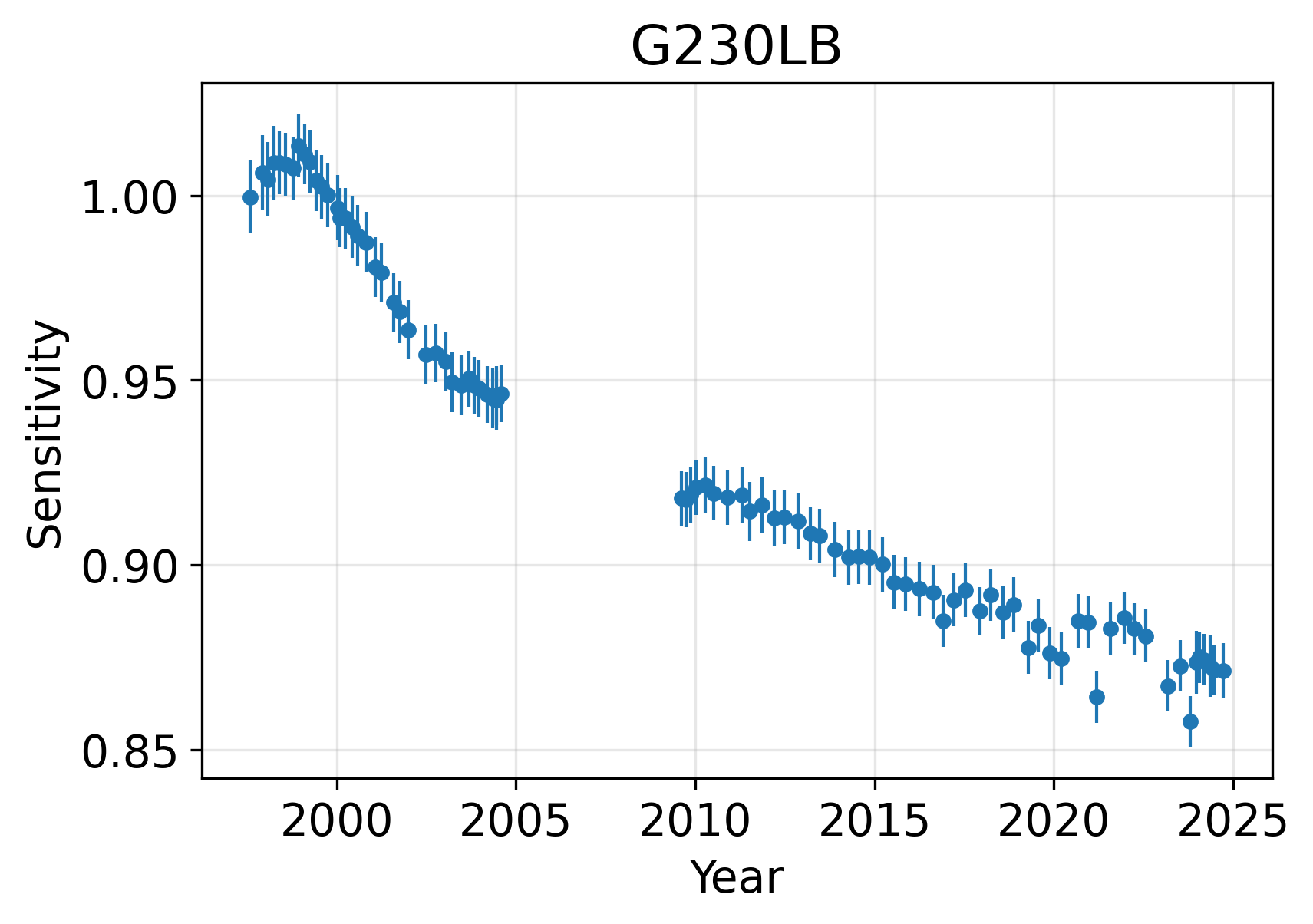
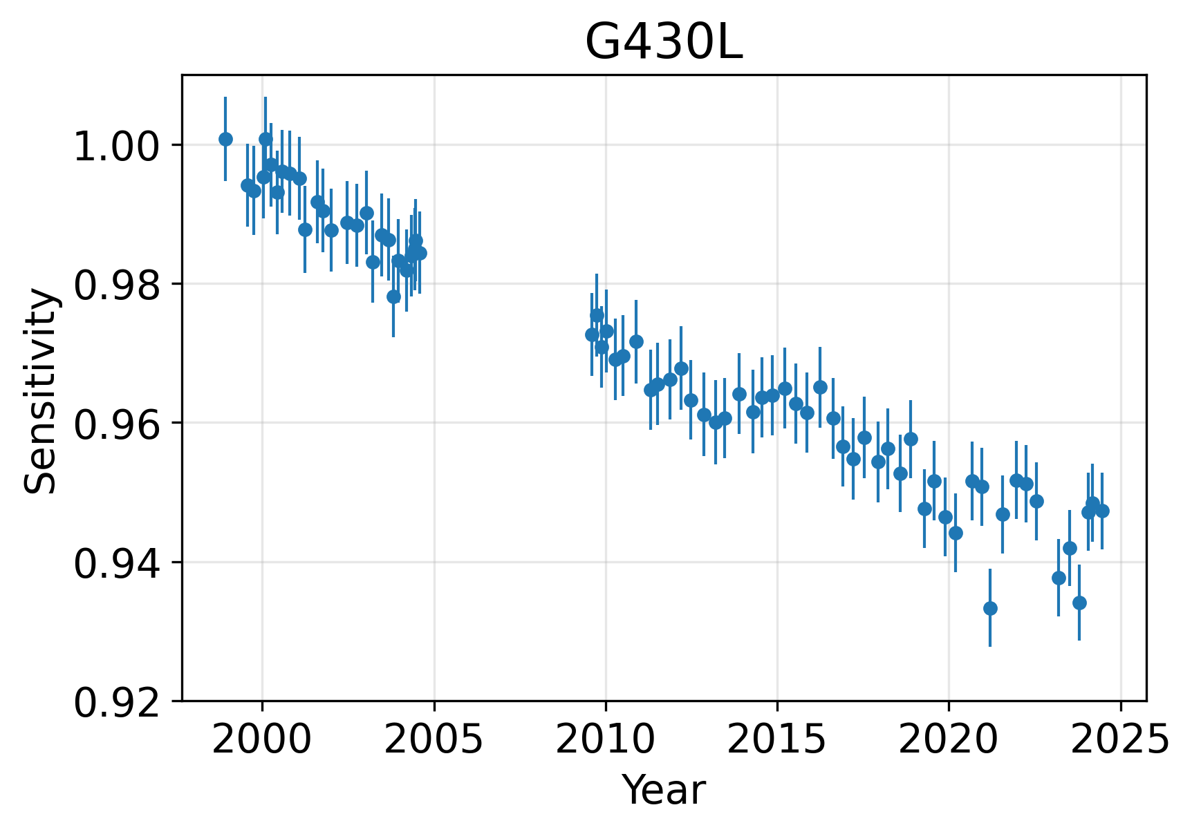
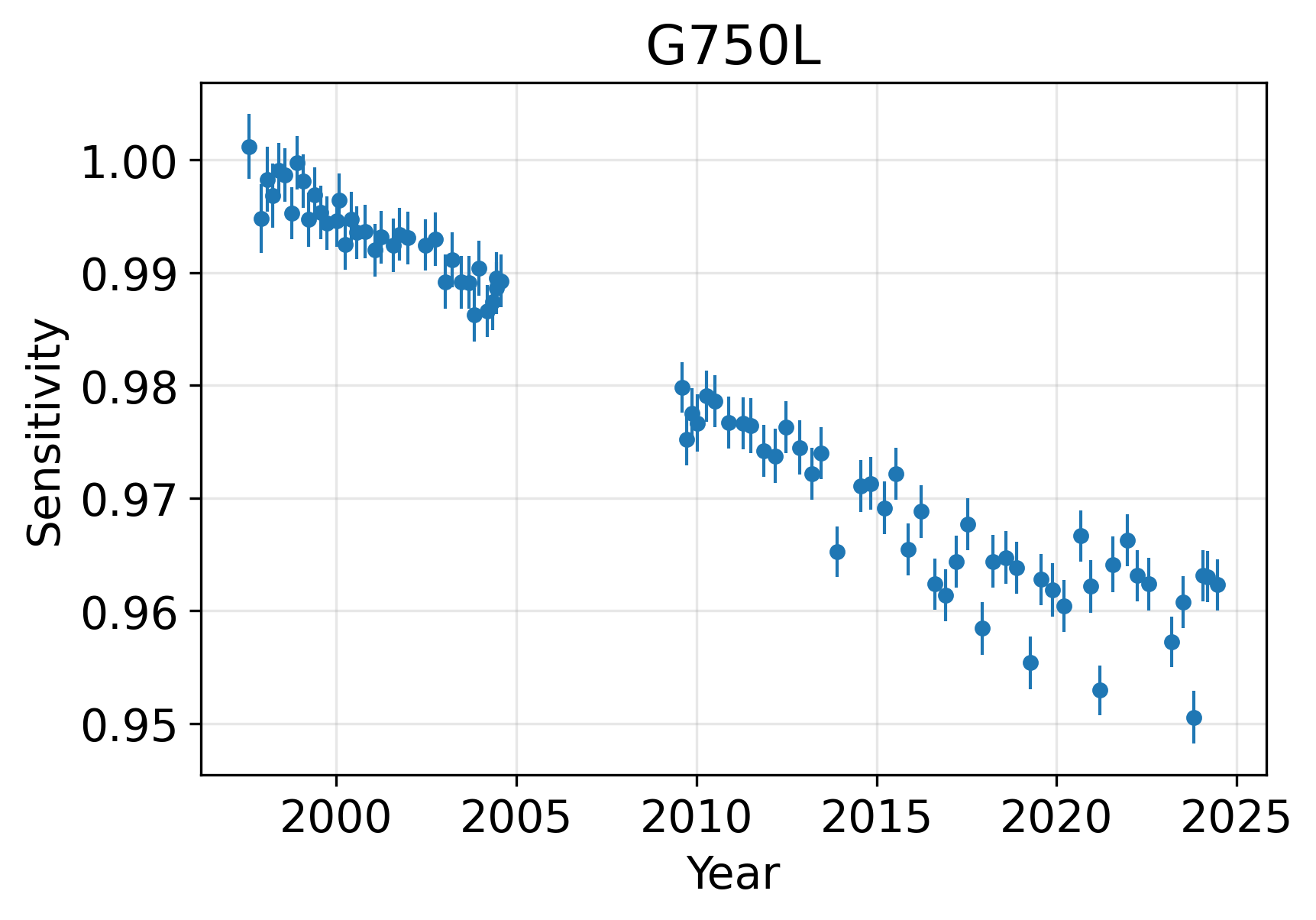
Trends for time-dependent sensitivity (TDS) for the CCD low-resolution (L) modes are shown in Figure 7.2. Sensitivities measured after SM4 are consistent with an extrapolation of the trends seen before the 2004 failure. Consistent with pre-failure trends, the sensitivity demonstrates a temperature dependence of +0.32, +0.21, and +0.06%/°C for G230LB, G430L, and G750L, respectively (see STIS ISR 2014-02). Selected wavelength settings of the medium-resolution (M) gratings G230MB, G430M, and G750M have also been monitored. Sensitivity trends measured for the limited M-mode wavelength coverage are similar to those observed in the L-modes at corresponding wavelengths. The G230LB and G230MB CCD configurations exhibit behavior similar to that found for the NUV-MAMA G230L mode (see Section 7.4.3), featuring an increase in sensitivity during the first 1.5 years of STIS operations, followed by decreasing sensitivity, with a slow-down in the decline beginning in early 2002 (see Figure 7.16).
TDS corrections for all CCD modes have been implemented into the STIS pipeline as TDSTAB reference files (see Section 15.1), and correct fluxes of extracted spectra for sensitivity changes to a typical accuracy of 1% or better. CTE corrections have also been implemented (see Section 7.3.7). The TDS trends are also incorporated into reference files used by Astropy's synphot and the STIS ETCs. This enables count rate predictions to take the sensitivity changes into account. The default TDS throughputs for synphot and STIS ETC calculations are extrapolated to their values for a date of April 2027.
Figure 7.2: Relative Wavelength-Averaged Sensitivity vs. Time for First-Order CCD L-Modes G230LB, G430L, and G750L.
7.2.6 CCD Long Wavelength Fringing
Like most CCDs, the STIS CCD exhibits fringing in the red, longward of ~7500 Å. This fringing limits the signal-to-noise routinely achievable in the red and NIR unless contemporaneous fringe flats are obtained (see below). In principle, fringing can also affect imaging observations if the source’s emission over the 50CCD or F28X50LP bandpass is dominated by emission lines redward of 7500 Å. However, if the bulk of the emission comes from blueward of 7500 Å, then emission from multiple wavelengths will smooth over the fringe pattern so that imaging will not be affected by fringing.
The amplitude of the fringes is a strong function of wavelength and spectral resolution. Table 7.2 lists the observed percent peak-to-peak and rms amplitudes of the fringes as a function of central wavelength for the G750M and G750L gratings. The listed "peak-to-peak" amplitudes are the best measure of the impact of the fringing on your data. The rms values at wavelengths <7000 Å give a good indication of the counting statistics in the flat-field images used for this analysis.
Table 7.2: Fringing Amplitude in Percent as a Function of Wavelength.
Wavelength (Å) |
|
|
|
|
6,100 | — | 1.21 | — | — |
6,250 | — | 1.23 | — | — |
6,600 | — | 1.23 | — | — |
6,750 | — | 1.29 | — | — |
7,250 | 4.62 | 1.52 | 3.18 | 2.13 |
7,750 | 9.61 | 3.10 | 8.58 | 3.08 |
8,250 | 10.53 | 3.26 | 6.76 | 2.80 |
8,750 | 14.83 | 3.85 | 10.81 | 3.98 |
9,250 | 27.16 | 9.00 | 23.42 | 7.92 |
9,750 | 32.09 | 10.78 | 25.35 | 8.96 |
10,250 | 18.23 | 6.04 | 17.30 | 5.89 |
The fringe pattern can be corrected by rectification with an appropriate flat field. The fringe pattern is a convolution of the contours of constant distance between the front and back surfaces of the CCD and the wavelength of the light on a particular part of the CCD. The fringe pattern has been shown to be very stable, as long as the wavelength of light on a particular part of the CCD stays constant. However, due to the grating wheel positioning uncertainty (Section 3.2.2, Slit and Grating Wheels) and the effect of temperature drifts in orbit, the wavelength on a particular part of the CCD will vary from observation to observation. Thus, the best de-fringing results are obtained by using a contemporaneous flat ("fringe flat"), i.e., a tungsten lamp flat taken at the same grating wheel setting and during the same orbit as your scientific exposures.
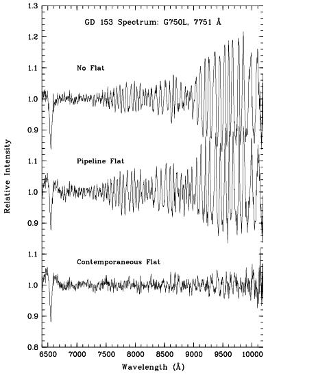
Table 7.3 compares the estimated peak-to-peak fringe amplitudes after flat-fielding by the library flat and those after flat fielding with an appropriately processed contemporaneous flat. These estimates are based upon actual measurements of spectra of both point sources and extended sources made during Cycle 7 (the results for point sources and extended sources were essentially the same). Figure 7.3 shows such a comparison for a G750L spectrum of a white dwarf; in this figure, the top panel shows white dwarf GD153 (central wavelength 7751 Å) with no flat-field correction, the second spectrum shows the result of de-fringing with the standard pipeline flat field, and the third spectrum shows the result of de-fringing with a contemporaneous flat (all spectra were divided by a smooth spline fit to the stellar continuum). It is clear that a contemporaneous flat provides a great improvement over the use of a library flat. Therefore, if you are observing in the far red (>7500 Å) and using grating G750L or G750M, you should take a contemporaneous flat field along with your scientific observations. More detailed information and analysis on fringe correction for STIS long-wavelength spectra can be found in STIS ISR 1998-19 and STIS ISR 1998-29. Tips for defringing spectra can be found in the July 2021 STAN, which includes references and examples for using the modern STIS Python package stistools.defringe.
Table 7.3: Residual Fringe Amplitude (rms, in percent) after Flat-Fielding with Library Pipeline Flat and a Contemporaneous Flat.
Wavelength |
|
|
|
|
7,500 | 3.0 | 1.2 | 4.0 | 0.9 |
7,750 | 2.5 | 1.3 | 5.3 | 0.8 |
8,000 | 4.2 | 1.3 | 7.5 | 1.0 |
8,250 | 4 | 1.0 | 5.3 | 0.9 |
8,500 | 5 | 0.9 | 8.3 | 1.0 |
8,750 | 6 | 0.9 | 6.5 | 0.9 |
9,000 | 8 | — | 8.3 | 1.0 |
9,250 | 10 | — | 17.5 | 1.4 |
9,500 | 11 | — | 18.7 | 2.0 |
9,750 | 12 | — | 19.7 | 2.4 |
10,000 | 10 | — | 11.7 | 2.4 |
1 Measurements of the fringe amplitude have not been made yet for G750M wavelength settings redward of 8561 Å. However, from our experience with fringe corrections we expect the residual fringe amplitudes to be of order 1% when contemporaneous fringe flats are used.
Figure 7.3: Comparison of De-fringing Capabilities of Reference File Flats and Those of Contemporaneous Flats.
7.2.7 Fringing Due to the Order Sorter Filters
Examination of long slit observations in the CCD spectroscopic modes has revealed periodic variations of intensity along the slit when highly monochromatic, calibration lamp sources are used. An example of such "chevron-pattern" variations is shown in Figure 7.4 and Figure 7.5. These variations are thought to be the result of transmission variations through the highly parallel faces of the order sorting filters that are situated next to the gratings in the optical path. In the cross dispersion direction, the modulation amplitude depends on the line width with a maximum of 13% for a monochromatic source in G430L and G430M modes, and 4.5% in G750L and G750M modes. Periods range from 40–80 pix/cycle. In the dispersion direction, there is a small, residual, high-frequency modulation with a peak amplitude of about 1.5% in G430M at the 5471 Å setting and with smaller amplitudes in all other modes and settings. No such modulation has been observed in any of the MAMA modes. Some modulation is also apparent in the CCD G230LB and G230MB modes, however the amplitudes of these modulations are much smaller.
Figure 7.4: An Example of the "Chevron Pattern" Variations.
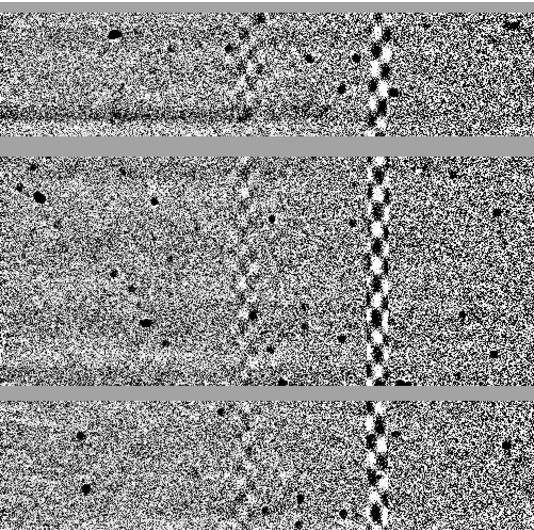
CCD image of a calibration lamp exposure which shows the chevron-pattern variations. The image is taken with the G430L grating and a 2 arcsecond slit. The chevron patterns are seen at the position of the emission lines.
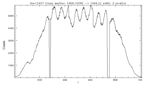
Figure 7.5: The 52X0.2 Slit Illumination Near 4269Å in Mode G430L Obtained with the Pt-Cr/Ne Calibration Lamp.
7.2.8 Optical Performance
Verification testing has shown that STIS meets its image-quality specifications. While the optics provide fine images at the focal plane, the detected point-spread functions (PSFs) are degraded somewhat more than expected by the CCD at wavelengths longward of about 7500 Å, where a broad halo appears, surrounding the PSF core. This halo is believed to be due to scatter within the CCD mounting substrate, which becomes more pronounced as the silicon transparency increases at long wavelengths. The effects of the red halo (see Figure 7.6), which extend to radii greater than 100 pixels (5 arcseconds), are not included in the encircled energies as a function of observing wavelength that are described for the CCD spectroscopic and imaging modes in Chapter 13 and 14, respectively. However, estimates of the encircled energy vs. radius that include the halo are shown in Table 7.4. The integrated energy in the halo amounts to approximately 20% of the total at 8050 Å and 30% at 9050 Å (see also STIS ISR 1997-13 for the implication for long-slit spectroscopic observations at long wavelengths). Note that the ACS WFC CCDs have a front-side metallization that reduces the large angle long wavelength halo problem in those detectors. This problem has been eliminated from the WFC3 CCD.
Table 7.4: Model of Encircled Energy Fraction as a Function of Wavelength for STIS CCD Imaging.
λ | Fraction in Central Pixel | Aperture Radius in Pixels | |||||||
(Å) | 2 | 5 | 10 | 15 | 19.7 | 39.4 | 59 | 118 | |
1,750 | 0.246 | 0.667 | 0.873 | 0.949 | 0.979 | 0.990 | 0.998 | 1.000 | 1.000 |
3,740 | 0.283 | 0.704 | 0.857 | 0.920 | 0.945 | 0.960 | 0.994 | 0.999 | 1.000 |
5,007 | 0.253 | 0.679 | 0.857 | 0.916 | 0.934 | 0.948 | 0.985 | 0.997 | 1.000 |
6,500 | 0.214 | 0.597 | 0.865 | 0.902 | 0.927 | 0.942 | 0.966 | 0.975 | 0.992 |
7,500 | 0.178 | 0.536 | 0.825 | 0.866 | 0.892 | 0.909 | 0.942 | 0.957 | 0.986 |
8,500 | 0.141 | 0.463 | 0.748 | 0.799 | 0.827 | 0.848 | 0.897 | 0.924 | 0.973 |
9,500 | 0.100 | 0.342 | 0.607 | 0.672 | 0.705 | 0.733 | 0.809 | 0.857 | 0.946 |
10,000 | 0.080 | 0.275 | 0.518 | 0.589 | 0.624 | 0.655 | 0.748 | 0.810 | 0.926 |
10,500 | 0.064 | 0.238 | 0.447 | 0.517 | 0.553 | 0.585 | 0.690 | 0.764 | 0.907 |
The CCD plate scale is 0.05072 arcsec/pix for imaging observations (see STIS ISR 2001-02), and in the spatial (across the dispersion) direction for spectroscopic observations. Due to the effect of anamorphic magnification, for spectroscopic observations the plate scale in the dispersion direction is slightly different and it depends on the grating used and its tilt. The plate scale in the dispersion direction ranges from 0.0512 to 0.0581 arcsec/pix (see STIS ISR 1998-23).
Figure 7.6: The Red Halo.
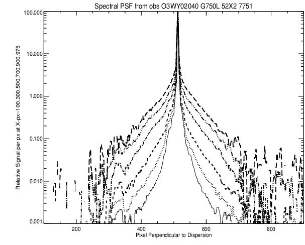
Cross-sections of the signal distribution perpendicular to the dispersion direction for G750L, at six wavelengths from 5752 Å to 10020 Å. Each PSF is normalized to a peak value of 100. The strong wavelength dependence of the PSF provides a clean separation of the curves.
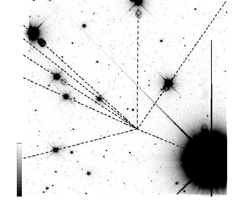
Figure 7.7: Ring-Shaped Ghost Images Near Bright Point Sources (50CCD Image).
7.2.9 Readout Format
A full detector readout is 1062 × 1044 pixels including physical and virtual overscans. Scientific data are obtained on 1024 × 1024 pixels, each projecting to ~0.05 × 0.05 arcseconds on the sky. For spectroscopic observations, the dispersion axis runs along AXIS1 (image X or along a row of the CCD), and the spatial axis of the slits runs along AXIS2 (image Y or along a column of the CCD). The CCD supports the use of subarrays to read out only a portion of the detector, and on-chip binning. For more details see Section 11.1.1.
7.2.10 Analog-to-Digital Conversion: Selecting the CCDGAIN
Electrons that accumulate in the CCD wells are read out and converted to data numbers (DN, the format of the output image) by the analog-to-digital converter at a default CCDGAIN of 1 e−/DN (i.e., every electron registers 1 DN). The CCD is also capable of operating at a gain of 4 e−/DN1. The analog-to-digital converter operates at 16 bits, producing a maximum of 65,536 DN/pix. This is not a limitation at either gain setting, because other factors set the maximum observable DN to lower levels in each case (see Section 7.3.2).
The CCDGAIN=1 setting has the lower read noise (Table 7.1) and digitization noise. Although the read noise has increased since the switch to the Side-2 electronics in July 2001 (see Section 7.2.2), CCDGAIN=1 is still the most appropriate setting for observations of faint sources. However, saturation occurs at about 33,000 e− at the CCDGAIN=1 setting (as described in Section 7.3.2).
The CCDGAIN=4 setting allows use of the entire CCD full well of 130,000 e−, and use of the CCDGAIN=4 setting is therefore recommended for imaging photometry of objects whenever more than 33,000 e− might be obtained in a single pixel of an individual sub-exposure. However, short exposures taken in CCDGAIN=4 show a large-scale pattern noise ("ripple") that is not removed by the standard bias images. This pattern noise is in addition to the usual coherent noise visible since STIS switched to using the backup Side-2 electronics. Figure 7.8 (a 0.2 second exposure of a lamp-illuminated small slit) shows an example of the CCDGAIN=4 ripple. The peak-to-peak intensities of these ripples vary from near zero to about 1 DN, and there is a large amount of coherence in the noise pattern. This coherence makes background determination difficult and limits the precision of photometry of faint objects in shallow exposures taken using CCDGAIN=4.
The CCD response when using CCDGAIN=4 remains linear even beyond the 130,000 e− full-well limit if one integrates over the pixels bled into (Section 7.3.2), and for specialized observations needing extremely high S/N, this property may be useful.
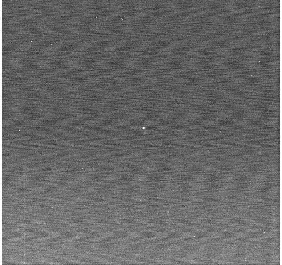
Figure 7.8: Ripple Effect in Short Exposures with CCDGAIN=4.
7.2.11 Long-term Rotational Drift
The CCD has been shown to undergo a long-term rotational drift, as evidenced by changes in both the spectral traces (STIS ISR 2007-03 - Dressel 2007) and the evolution of the STIS CCD flat fields (STIS ISR 2022-01 - Ward-Duong 2022).
In particular, ISR 2007-03 analyzed the CCD spectral traces of standard stars observed with various L and M mode settings. The study found rotation rates of 0.0031 \pm 0.0003 deg/yr for G230LB, 0.0041 \pm 0.0001 deg/yr for G430L, and 0.0037 \pm 0.0003 deg/yr for G750L—values consistent within 3σ—and in the range 0.0041–0.0053 deg/yr for G750M (6581, 6768, 8561). These rotation rates were recorded in the DEGPERYR column of the 1-D Spectrum Trace reference file. ISR 2022-01, on the other hand, measured the rotation of dust motes in 50CCD flat fields over a 20-year time span, finding a rotational drift rate of 0.0031 \pm 0.0001 deg/yr. These results are further supported by an independent study that reported a rotation rate of approximately 0.004 deg/yr based on the STIS 50CCD and 50CORON apertures (Nguyen et al. 2021).
Currently, rotation corrections are applied to the subset of M and L modes analyzed in ISR 2007-03, while no correction is made to CCD data to account for the long-term rotational evolution of the flat fields. Ongoing efforts aim to assess the broader impact of this rotation on other aspects of the CCD, including the calibration accuracy of data obtained at the E1 aperture position and the accuracy of coronagraphic aperture locations listed in the STIS Science Instrument Aperture File (SIAF). Further updates will be implemented as these assessments progress.
1 Measurement of the CCDGAIN=4 to CCDGAIN=1 ratio after SM4 finds that CCDGAIN=4 actually corresponds to 4.087 ± 0.007 e−/DN. See STIS ISR 2017-05.
-
STIS Instrument Handbook
- • Acknowledgments
- Chapter 1: Introduction
-
Chapter 2: Special Considerations for Cycle 34
- • 2.1 Impacts of Reduced Gyro Mode on Planning Observations
- • 2.2 STIS Performance Changes Pre- and Post-SM4
- • 2.3 New Capabilities for Cycle 34
- • 2.4 Use of Available-but-Unsupported Capabilities
- • 2.5 Choosing Between COS and STIS
- • 2.6 Scheduling Efficiency and Visit Orbit Limits
- • 2.7 MAMA Scheduling Policies
- • 2.8 Prime and Parallel Observing: MAMA Bright-Object Constraints
- • 2.9 STIS Snapshot Program Policies
- Chapter 3: STIS Capabilities, Design, Operations, and Observations
- Chapter 4: Spectroscopy
- Chapter 5: Imaging
- Chapter 6: Exposure Time Calculations
- Chapter 7: Feasibility and Detector Performance
-
Chapter 8: Target Acquisition
- • 8.1 Introduction
- • 8.2 STIS Onboard CCD Target Acquisitions - ACQ
- • 8.3 Onboard Target Acquisition Peakups - ACQ PEAK
- • 8.4 Determining Coordinates in the International Celestial Reference System (ICRS) Reference Frame
- • 8.5 Acquisition Examples
- • 8.6 STIS Post-Observation Target Acquisition Analysis
- Chapter 9: Overheads and Orbit-Time Determination
- Chapter 10: Summary and Checklist
- Chapter 11: Data Taking
-
Chapter 12: Special Uses of STIS
- • 12.1 Slitless First-Order Spectroscopy
- • 12.2 Long-Slit Echelle Spectroscopy
- • 12.3 Time-Resolved Observations
- • 12.4 Observing Too-Bright Objects with STIS
- • 12.5 High Signal-to-Noise Ratio Observations
- • 12.6 Improving the Sampling of the Line Spread Function
- • 12.7 Considerations for Observing Planetary Targets
- • 12.8 Special Considerations for Extended Targets
- • 12.9 Parallel Observing with STIS
- • 12.10 Coronagraphic Spectroscopy
- • 12.11 Coronagraphic Imaging - 50CORON
- • 12.12 Spatial Scans with the STIS CCD
-
Chapter 13: Spectroscopic Reference Material
- • 13.1 Introduction
- • 13.2 Using the Information in this Chapter
-
13.3 Gratings
- • First-Order Grating G750L
- • First-Order Grating G750M
- • First-Order Grating G430L
- • First-Order Grating G430M
- • First-Order Grating G230LB
- • Comparison of G230LB and G230L
- • First-Order Grating G230MB
- • Comparison of G230MB and G230M
- • First-Order Grating G230L
- • First-Order Grating G230M
- • First-Order Grating G140L
- • First-Order Grating G140M
- • Echelle Grating E230M
- • Echelle Grating E230H
- • Echelle Grating E140M
- • Echelle Grating E140H
- • PRISM
- • PRISM Wavelength Relationship
-
13.4 Apertures
- • 52X0.05 Aperture
- • 52X0.05E1 and 52X0.05D1 Pseudo-Apertures
- • 52X0.1 Aperture
- • 52X0.1E1 and 52X0.1D1 Pseudo-Apertures
- • 52X0.2 Aperture
- • 52X0.2E1, 52X0.2E2, and 52X0.2D1 Pseudo-Apertures
- • 52X0.5 Aperture
- • 52X0.5E1, 52X0.5E2, and 52X0.5D1 Pseudo-Apertures
- • 52X2 Aperture
- • 52X2E1, 52X2E2, and 52X2D1 Pseudo-Apertures
- • 52X0.2F1 Aperture
- • 0.2X0.06 Aperture
- • 0.2X0.2 Aperture
- • 0.2X0.09 Aperture
- • 6X0.2 Aperture
- • 0.1X0.03 Aperture
- • FP-SPLIT Slits 0.2X0.06FP(A-E) Apertures
- • FP-SPLIT Slits 0.2X0.2FP(A-E) Apertures
- • 31X0.05ND(A-C) Apertures
- • 0.2X0.05ND Aperture
- • 0.3X0.05ND Aperture
- • F25NDQ Aperture
- 13.5 Spatial Profiles
- 13.6 Line Spread Functions
- • 13.7 Spectral Purity, Order Confusion, and Peculiarities
- • 13.8 MAMA Spectroscopic Bright Object Limits
-
Chapter 14: Imaging Reference Material
- • 14.1 Introduction
- • 14.2 Using the Information in this Chapter
- 14.3 CCD
- 14.4 NUV-MAMA
-
14.5 FUV-MAMA
- • 25MAMA - FUV-MAMA, Clear
- • 25MAMAD1 - FUV-MAMA Pseudo-Aperture
- • F25ND3 - FUV-MAMA
- • F25ND5 - FUV-MAMA
- • F25NDQ - FUV-MAMA
- • F25QTZ - FUV-MAMA, Longpass
- • F25QTZD1 - FUV-MAMA, Longpass Pseudo-Aperture
- • F25SRF2 - FUV-MAMA, Longpass
- • F25SRF2D1 - FUV-MAMA, Longpass Pseudo-Aperture
- • F25LYA - FUV-MAMA, Lyman-alpha
- • 14.6 Image Mode Geometric Distortion
- • 14.7 Spatial Dependence of the STIS PSF
- • 14.8 MAMA Imaging Bright Object Limits
- Chapter 15: Overview of Pipeline Calibration
- Chapter 16: Accuracies
-
Chapter 17: Calibration Status and Plans
- • 17.1 Introduction
- • 17.2 Ground Testing and Calibration
- • 17.3 STIS Installation and Verification (SMOV2)
- • 17.4 Cycle 7 Calibration
- • 17.5 Cycle 8 Calibration
- • 17.6 Cycle 9 Calibration
- • 17.7 Cycle 10 Calibration
- • 17.8 Cycle 11 Calibration
- • 17.9 Cycle 12 Calibration
- • 17.10 SM4 and SMOV4 Calibration
- • 17.11 Cycle 17 Calibration Plan
- • 17.12 Cycle 18 Calibration Plan
- • 17.13 Cycle 19 Calibration Plan
- • 17.14 Cycle 20 Calibration Plan
- • 17.15 Cycle 21 Calibration Plan
- • 17.16 Cycle 22 Calibration Plan
- • 17.17 Cycle 23 Calibration Plan
- • 17.18 Cycle 24 Calibration Plan
- • 17.19 Cycle 25 Calibration Plan
- • 17.20 Cycle 26 Calibration Plan
- • 17.21 Cycle 27 Calibration Plan
- • 17.22 Cycle 28 Calibration Plan
- • 17.23 Cycle 29 Calibration Plan
- • 17.24 Cycle 30 Calibration Plan
- • 17.25 Cycle 31 Calibration Plan
- • 17.26 Cycle 32 Calibration Plan
- • 17.27 Cycle 33 Calibration Plan
- Appendix A: Available-But-Unsupported Spectroscopic Capabilities
- • Glossary