7.8 Specifying Orientation on the Sky
HRC has been unavailable since January 2007. Information about the HRC is provided for archival purposes.
WFC may be offered as shared risk in Cycle 34 and receive minimal support and calibration. See the ACS website, Call for Proposals, and OPCR webpage for the latest status.
Determining the orientation of an image requires knowledge of the telescope roll and the angle of the aperture relative to the HST coordinate frame. A target may need to be oriented in a preferred direction on a detector, for instance when spectroscopy is to be performed, or to avoid certain scattered light artifacts (see Section 4.5 of the Data Handbook).
To specify an ORIENT in a Phase II, use the ORIENT selection in APT. Keep in mind that this parameter is just the Position Angle (PA) of the HST U3 axis, which is the inverse of V3, as seen Figure 3.1 and Figure 7.9 in this Handbook and the Phase II Proposal Instructions. APT provides a convenient interactive display of the aperture and orientations in your field. The ORIENT parameter is related to the following discussion of ACS geometry.
All HST aperture positions and orientations are defined within an orthogonal Euler angle coordinate system that is labeled V1, V2, and V3, in which V1 is nominally along the telescope roll axis, which is the same as the optical axis. The location of all apertures are therefore defined in the (V2, V3) plane. For more information about HST instrument aperture locations and axes in the HST field of view (FoV), please visit the HST FoV Geometry webpage.
The V3 position angle (PA_V3 in Figure 7.8) is defined as the angle of the projection of the V3 axis on the sky, measured from North to East with the aperture denoting the origin. This is almost identical to the telescope roll angle. There is a small difference between roll angles measured at the V1 axis and those measured at the aperture, as the (V2, V3) system is spherical (see ACS TIR 2014-021 for more detailed explanation). Due to the fact that ACS is far from the optical axis, this 3-dimensional correction can amount to several tenths of a degree depending on the target declination. In the (V2, V3) coordinate system, as shown in Figure 7.8, aperture orientations are defined by the angles their x and y axes make with the V3 axis, ßx and ßy, measured in an anticlockwise direction (the value of ßx as illustrated in Figure 7.8 would be considered negative). Hence, the angles these axes make with North are found by adding the axis angles to the position angle.
Figure 7.8: Aperture and image feature orientation.
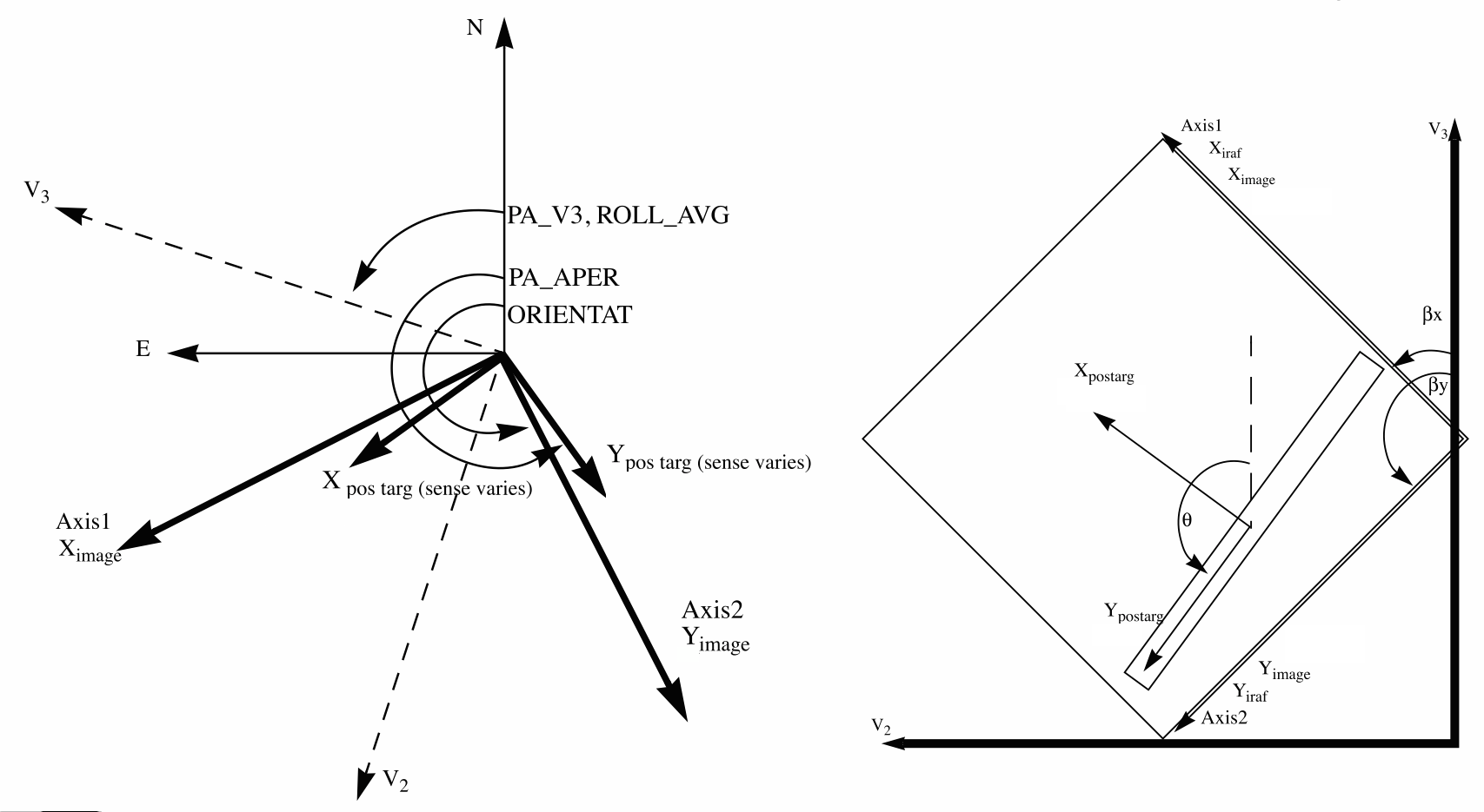
The figure accurately describes ORIENTAT and PA_APER. All of the orientations are taken from the HST FoV Geometry webpage.
ORIENTAT, the angle the detector y axis makes with North, which is equal to p + ßy, where p is the angle from North relative to V3 and ßy is the angle of the y axis of the detector relative to V3. Another angle keyword supplied is PA_APER, which is the angle the aperture y axis makes with North. Both angles are defined at the aperture so using them does not involve the displacement difference. Normally, the aperture and detector y axes are parallel, and so PA_APER = ORIENTAT. Several STIS slit apertures were not aligned parallel to the detector axes, so this distinction was meaningful, but ACS has no slit apertures so this difference will probably not arise in almost all science cases. In any case, we recommend using PA_APER in Phase II's (see Section 7.8.1).Beyond establishing the direction of the aperture axes, it will often be necessary to know the orientation of a feature, such as the plane of a galaxy, within an image. Conversely, we need to know what direction within an image corresponds to North. To this end we define a feature angle α within the aperture as measured on the science image, anti-clockwise from the y axis so that it is in the same sense as the previously defined angles. For an orthogonal set of aperture axes, the direction of this feature would be PA_APER + α, and the image direction of North would be the value of α which makes this angle zero, namely −PA_APER, still measured in an anti-clockwise direction from the y axis.
Figure 7.9: ACS apertures in the V2/V3 reference frame.
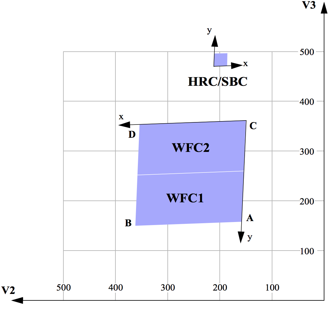
The readout amplifiers (A,B,C,D) are indicated on the figure. The WFC data products from the calibration pipeline will be oriented so that WFC1 (chip 1, which uses amplifiers A and B) is on top. The HRC data products are also oriented such that amps A and B are on top, but they are inverted from WFC images with respect to the sky.
| (1) | V2 = V2_r + s_x \sin \beta_x (x - x_r) + s_y \sin \beta_y (y - y_r) |
| (2) | V3 = V3_r + s_x \cos \beta_x (x - x_r) + s_y \cos \beta_y (y - y_r) |
where xr and yr are the origin of the image coordinates, sx and sy are scales in arcseconds per pixel along the image x and y axes, V2r and V3r are the origin of the aperture coordinates (but they do not enter into the angle calculations as they are fixed in the system). Note that x and y coordinates should be corrected for geometric distortion before the transformation is applied.
For the ACS apertures, the values in Table 7.11 have been derived from results of operating the ACS in the Refractive Aberrated Simulator. These should not be considered as true calibrations but they indicate some aperture features, such as the non-orthogonality of the aperture axes, and the x and y scale differences for HRC and SBC. Note that the values in Table 7.11 are also retrievable from the headers of the science images.
Table 7.11: Plate scales and axis angles for the 3 ACS channels.
Aperture | xr | yr | V2r | V3r | sx | sy | βx | βy | βx−βy |
|---|---|---|---|---|---|---|---|---|---|
WFC1 | 2124 | 1024 | 264.21 | 198.55 | 0.049313 | 0.048651 | 92.46 | 177.35 | –84.89 |
WFC2 | 2124 | 1024 | 259.97 | 302.48 | 0.049895 | 0.050328 | 91.7 | 177.78 | –86.08 |
SBC | 512 | 400 | 205 | 467 | 0.033658 | 0.030009 | –84.56 | –0.05 | –84.51 |
HRC | 531 | 512 | 206 | 472 | 0.028431 | 0.024843 | –84.12 | 0.08 | –84.2 |
Figure 7.9 shows that a rotation from x to y is in the opposite sense to a rotation from V2 to V3. This will be the arrangement for ACS apertures. This is significant in defining the sense of the rotation angles. For a direction specified by displacements Δx and Δy in the image, the angle α is arctan(−Δx/Δy).
Because of the oblique coordinates, the angle αs on the sky will not be equal to α. To calculate the sky angle, it is convenient to define another set of orthogonal axes (xs, ys), similar to the (V2, V3) but rotated so that ys lies along y, and xs is approximately in the x direction. Let ω = βy − βx be the angle between the projected detector axes and let their origins be coincident, for simplicity. Then the transformation is:
| (3) | x_s = s_x \sin \omega x |
| (4) | y_s = s_x \cos \omega x + s_y y |
By comparing differentials and defining αs as arctan(−Δxs/Δys) we find:
| (5) | \tan \alpha_s = \frac{s_x \sin \omega \sin \alpha}{s_y \cos \alpha - s_x \cos \omega \sin \alpha} |
The equation as written will place the angle in the proper quadrant if the Fortran atan2 function, the IDL atan function, or the Python atan2 function is used. To get the true angle East of North, for a feature seen at angle α in the image, calculate αs, and add to PA_APER.
The inverse relation is
| (6) | \tan \alpha = \frac{s_y \sin \alpha_s}{s_x \sin(\alpha_s + \omega)}. |
To find the value of α corresponding to North, we need the value of αs such that PA_APER + αs = 0. This guarantees that the reference frame is correctly oriented. To do this, substitute −PA_APER for αs in the equation to get the angle α in the image that corresponds to North. The values of the pixel scales for all instruments can be found on the Drizzlepac website. The axis angles for all instruments are found on the HST FoV Geometry webpage.
7.8.1 Determining Orientation for Phase II
A particular orientation is specified in an HST Phase II proposal using yet another coordinate system: (U2, U3). In this system, the U2 and U3 axes are opposite to V2 and V3, so, for example, U3 = −V3. The angle ORIENT, used in a Phase II proposal to specify a particular HST orientation, is the position angle of U3 measured from North towards East. This means the direction of the V3 axis with respect to North is PA_APER − βy and so
| (7) | \texttt{ORIENT} = \texttt{PA_APER} - \beta_y \pm 180^{\circ} |
This orientation can be checked by using APT, specifying the orientation, and then viewing in Aladin.
1TIRs available upon request.
-
ACS Instrument Handbook
- • Acknowledgments
- • Change Log
- • Chapter 1: Introduction
- Chapter 2: Considerations and Changes After SM4
- Chapter 3: ACS Capabilities, Design and Operations
- Chapter 4: Detector Performance
- Chapter 5: Imaging
- Chapter 6: Polarimetry, Coronagraphy, Prism and Grism Spectroscopy
-
Chapter 7: Observing Techniques
- • 7.1 Designing an ACS Observing Proposal
- • 7.2 SBC Bright Object Protection
- • 7.3 Operating Modes
- • 7.4 Patterns and Dithering
- • 7.5 A Road Map for Optimizing Observations
- • 7.6 CCD Gain Selection
- • 7.7 ACS Apertures
- • 7.8 Specifying Orientation on the Sky
- • 7.9 Parallel Observations
- • 7.10 Pointing Stability for Moving Targets
- Chapter 8: Overheads and Orbit-Time Determination
- Chapter 9: Exposure-Time Calculations
-
Chapter 10: Imaging Reference Material
- • 10.1 Introduction
- • 10.2 Using the Information in this Chapter
-
10.3 Throughputs and Correction Tables
- • WFC F435W
- • WFC F475W
- • WFC F502N
- • WFC F550M
- • WFC F555W
- • WFC F606W
- • WFC F625W
- • WFC F658N
- • WFC F660N
- • WFC F775W
- • WFC F814W
- • WFC F850LP
- • WFC G800L
- • WFC CLEAR
- • HRC F220W
- • HRC F250W
- • HRC F330W
- • HRC F344N
- • HRC F435W
- • HRC F475W
- • HRC F502N
- • HRC F550M
- • HRC F555W
- • HRC F606W
- • HRC F625W
- • HRC F658N
- • HRC F660N
- • HRC F775W
- • HRC F814W
- • HRC F850LP
- • HRC F892N
- • HRC G800L
- • HRC PR200L
- • HRC CLEAR
- • SBC F115LP
- • SBC F122M
- • SBC F125LP
- • SBC F140LP
- • SBC F150LP
- • SBC F165LP
- • SBC PR110L
- • SBC PR130L
- • 10.4 Geometric Distortion in ACS
- • Glossary