7.7 IR Exposure and Readout
The general operating modes of IR detectors have been described in Chapter 5. In this section we will detail the readout modes implemented in WFC3.
7.7.1 Exposure Time
Unlike the UVIS channel, the IR channel does not have a mechanical shutter. Integration times are thus determined purely electronically, by resetting the charge on the detector, and then accumulating signal until the exposure is completed. A second major difference from the UVIS channel is that the IR detector is read out non-destructively as the exposure accumulates, as opposed to the single destructive readout at the end of a CCD exposure.
There are pre-defined accumulation and readout sequences available to IR observers, which are used to set the total exposure time as described in the next subsection.
7.7.2 MULTIACCUM Mode
In IR observing it is possible, and desirable, to sample the signal multiple times as an exposure accumulates, and the MULTIACCUM mode accomplishes this. MULTIACCUM is the only observing mode available for the IR channel.
Multiple readouts offer three major advantages. First, the multiple reads provide a way to record a signal in a pixel before it saturates, thus effectively increasing the dynamic range of the final image. Second, the multiple reads can be analyzed to isolate and remove cosmic-ray events. Third, fitting to multiple reads provides a means for reducing the net effective read noise, which is relatively high for the IR detector.
The disadvantage of multiple readouts is that they are data-intensive. The HgCdTe detector array is 1024 × 1024 pixels, which is only about 1/16 by pixel number of the 4096 × 4102 UVIS array. However, since up to 16 IR readouts are used, the total data volume of a single IR exposure approaches that of a single UVIS frame. A maximum of 32 IR full array readouts can be stored in the instrument buffer, after which the content of the buffer must be dumped to the HST Solid State Recorder (SSR). A buffer dump of 16 full array reads takes about 5.8 minutes.
MULTIACCUM readout consists of the following sequence of events:
- Array reset: After a fast calibration of the analog-to-digital converters, all pixels are set to the detector bias level via two rapid reset cycles of the entire chip.
- Array read: The charge in each pixel is measured and stored in the on-board computer's memory. This is done as soon as practical after the second array reset in step 1. In effect, given the short delay and the time needed to read the array, a very short-exposure image is stored in memory. This is known as the zero read.
- Multiple integration-read cycles: The detector integrates for a certain amount of time and then the charge in each pixel is read out. This step can be repeated up to a total of 15 times following the zero read during the exposure. All frames are individually stored in the on-board computer memory. Note that it takes a finite time (2.93 sec) to read the full array, so there is a time delay between reading the first and last pixel. Because this delay is constant for each read, it cancels out in difference images.
- Return to idle mode: The detector returns to idle mode, where it is continuously flushed in order to prevent charge build-up and to limit the formation of residual images.
All sequences start with the same “reset, reset, read, read” sequence, where the two reads are done as quickly as possible. This “double reset read” was originally implemented because the very first read after the reset may show an offset that does not reproduce in the following reads.
7.7.3 MULTIACCUM Timing Sequences: Full Array Apertures
There are 12 pre-defined sample sequences, optimized to cover a wide range of observing situations, available for the full-frame IR apertures. (See Section 7.7.4 for a discussion of the sample sequences available for the IR subarray apertures. The same names are used for the sample sequences, but the times are different.) The maximum number of reads (following the zero read) during an exposure is 15, which are collected as the signal ramps up. It is possible to select less than 15 reads, thus cutting the ramp short and reducing the total exposure time. However, the timing of the individual reads within any of the 12 sequences cannot be adjusted by the user. This approach has been adopted as the optimal calibration of IR detectors requires a dedicated set of reference files (e.g., dark frames) for each timing pattern.
In summary, a WFC3/IR exposure is fully specified by choosing:
- one of the 12 available pre-defined timing sequences, and
- the total number of samples (NSAMP, which must be no more than 15), which determines the total exposure time
The 11 timing sequences for the IR channel are:
- One RAPID sequence: the detector is sampled with the shortest possible time interval between reads.
- Six linear (SPARS) sequences: the detector is sampled with uniform time intervals between reads, a so-called “linear sample up the ramp.” (“SPARS” is a contraction of the word “sparse.”)
- Five rapid-log-linear (STEP) sequences: the detector is initially sampled with the shortest possible time interval between reads, then uses logarithmically spaced reads to transition to a sequence of uniform samples.
All 12 of the sequences above refer to readouts of the full 1024 × 1024 detector array. See Section 7.7.4 below for the timing sequences available for subarrays. Details of the sequences are in the following paragraphs. The timings of the individual reads are given in Table 7.8.
RAPID Sequence
The RAPID sequence provides linear sampling at the fastest possible speed. For the full array, this equates to one frame every 2.9 s, and the entire set of 16 reads completed in less than 44 s. The RAPID mode is mainly intended for the brightest targets. Due to the overheads imposed by buffer dumps (see Chapter 10), observations in this mode done continuously would have low observing efficiency.
SPARS Sequences
The SPARS sequences use evenly spaced time intervals between reads. The six available SPARS sequences are designated SPARS5, SPARS10, SPARS25, SPARS50, SPARS100 and SPARS200, corresponding to sampling intervals of approximately 5, 10, 25, 50, 100, and 200 s, respectively.
The SPARS modes can be regarded as the most basic readout modes, and they are applicable to a wide range of target fluxes. They provide flexibility in integration time and are well-suited to fill an orbital visibility period with several exposures.
SPARS5, introduced during cycle 23, has time steps intermediate between those of RAPID and SPARS10. It is especially useful for spatially scanned grism observations of bright stars (see Section 8.6) with subarray apertures (see Section 7.7.4).
STEP Sequences
The five available rapid-logarithmic-linear sequences are STEP25, STEP50, STEP100, STEP200, and STEP400. They begin with linear spacing (the same as the RAPID sequence), continue with logarithmic spacing up to the given number of seconds (e.g., 50 s for STEP50), and then conclude with linear spacing in increments of the given number of seconds for the remainder of the sequence. See Figure 7.10 for an illustration of a STEP sequence.
The STEP mode is intended to provide a more uniform sampling across a wide range of stellar magnitudes, which is especially important for imaging fields containing both faint and bright targets. The faint targets require a long, linearly sampled integration, while the bright targets need to be sampled several times early in the exposure, before they saturate. Thus, the dynamic range of the final image is increased.
Figure 7.10: Example of STEP sequence with NSAMP=4. NSAMP+1 images are stored in the observer’s FITS image
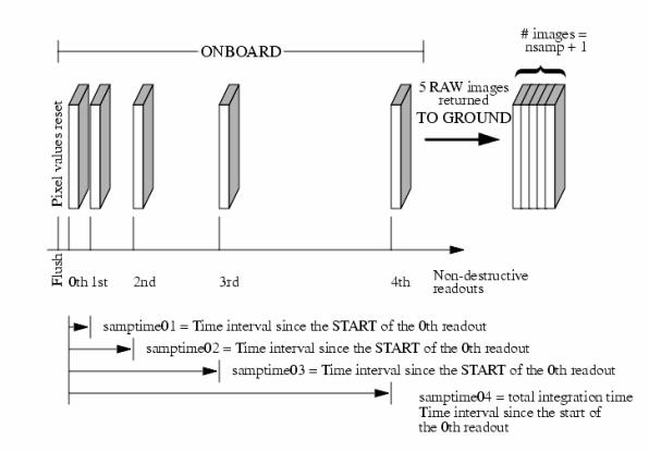
Table 7.8: Sample times of 1024 × 1024 MULTIACCUM readouts in seconds (this information is also in Table 13.4 of the Phase II Proposal Instructions).
NSAMP | RAPID | SPARS (sec) | |||||
|---|---|---|---|---|---|---|---|
SPARS5 | SPARS10 | SPARS25 | SPARS50 | SPARS100 | SPARS200 | ||
1 | 2.932 | 2.932 | 2.932 | 2.932 | 2.932 | 2.932 | 2.932 |
2 | 5.865 | 7.933 | 12.933 | 27.933 | 52.933 | 102.933 | 202.932 |
3 | 8.797 | 12.934 | 22.934 | 52.933 | 102.933 | 202.933 | 402.932 |
4 | 11.729 | 17.935 | 32.935 | 77.934 | 152.934 | 302.933 | 602.932 |
5 | 14.661 | 22.935 | 42.936 | 102.934 | 202.934 | 402.934 | 802.933 |
6 | 17.594 | 27.936 | 52.937 | 127.935 | 252.935 | 502.934 | 1002.933 |
7 | 20.526 | 32.937 | 62.938 | 152.935 | 302.935 | 602.934 | 1202.933 |
8 | 23.458 | 37.938 | 72.939 | 177.936 | 352.935 | 702.935 | 1402.933 |
9 | 26.391 | 42.938 | 82.940 | 202.936 | 402.936 | 802.935 | 1602.933 |
10 | 29.323 | 47.939 | 92.941 | 227.937 | 452.936 | 902.935 | 1802.933 |
11 | 32.255 | 52.940 | 102.942 | 252.937 | 502.937 | 1002.936 | 2002.933 |
12 | 35.187 | 57.941 | 112.943 | 277.938 | 552.937 | 1102.936 | 2202.933 |
13 | 38.120 | 62.942 | 122.944 | 302.938 | 602.938 | 1202.936 | 2402.933 |
14 | 41.052 | 67.942 | 132.945 | 327.939 | 652.938 | 1302.936 | 2602.933 |
15 | 43.984 | 72.943 | 142.946 | 352.940 | 702.939 | 1402.937 | 2802.933 |
NSAMP | RAPID | STEP (sec) | |||||
STEP25 | STEP50 | STEP100 | STEP200 | STEP400 | |||
1 | 2.932 | 2.932 | 2.932 | 2.932 | 2.932 | 2.932 | |
2 | 5.865 | 5.865 | 5.865 | 5.865 | 5.865 | 5.865 | |
3 | 8.797 | 8.797 | 8.797 | 8.797 | 8.797 | 8.797 | |
4 | 11.729 | 11.729 | 11.729 | 11.729 | 11.729 | 11.729 | |
5 | 14.661 | 24.230 | 24.230 | 24.230 | 24.230 | 24.230 | |
6 | 17.594 | 49.230 | 49.230 | 49.230 | 49.230 | 49.230 | |
7 | 20.526 | 74.231 | 99.231 | 99.231 | 99.231 | 99.231 | |
8 | 23.458 | 99.231 | 149.231 | 199.231 | 199.231 | 199.231 | |
9 | 26.391 | 124.232 | 199.232 | 299.231 | 399.231 | 399.231 | |
10 | 29.323 | 149.232 | 249.232 | 399.232 | 599.231 | 799.232 | |
11 | 32.255 | 174.233 | 299.232 | 499.232 | 799.231 | 1199.232 | |
12 | 35.187 | 199.233 | 349.233 | 599.232 | 999.231 | 1599.233 | |
13 | 38.120 | 224.234 | 399.233 | 699.233 | 1199.231 | 1999.233 | |
14 | 41.052 | 249.234 | 449.234 | 799.233 | 1399.231 | 2399.234 | |
15 | 43.984 | 274.235 | 499.234 | 899.233 | 1599.231 | 2799.235 | |
7.7.4 MULTIACCUM Timing Sequences: Subarray Apertures
As described in Section 7.4.4, subarrays are available in order to reduce data volume and enable short exposure times, defined in sample sequences. For a given sample sequence name, the sample times are shorter for smaller subarrays. Note that only certain combinations of subarrays and sample sequences are supported by STScI. Other MULTIACCUM sequences can be used in principle but are not supported, and additional calibration observations would have to be made by the observer. The supported combinations are presented in Table 7.9. The exposure times may be found in the Phase II Proposal Instructions, Chapter 12 (Wide Field Camera 3).
SPARS5, introduced during Oct 2015 (cycle 23), is especially useful for spatially scanned grism observations of bright stars (see Section 8.6).
Certain combinations of IR subarrays and sample sequences give rise to images containing a sudden low-level jump in the overall background level of the image. Observers can avoid this effect by ordering image sizes within a visit from large to small (see Section 7.4.4).
Table 7.9: Supported subarray sample sequences.
Aperture | Sample Sequence | ||||
RAPID | SPARS5 | SPARS10 | SPARS25 | STEP25 | |
IRSUB64 | yes | no | no | no | no |
IRSUB64-FIX | yes | no | no | no | no |
IRSUB128 | yes | no | yes | no | no |
IRSUB128-FIX | yes | no | yes | no | no |
IRSUB256 | yes | yes | yes | yes | no |
IRSUB256-FIX | yes | yes | yes | yes | no |
IRSUB512 | yes | yes | no | yes | yes |
IRSUB512-FIX | yes | yes | no | yes | yes |
See Section 12.3.1 of the Phase II Proposal Instructions, Tables 12.6 to 12.7, for the sample times associated with each combination of sample sequence and subarray size. Note that the sample times for a given sample sequence name are shorter for smaller subarrays. |
-
WFC3 Instrument Handbook
- • Acknowledgments
- Chapter 1: Introduction to WFC3
- Chapter 2: WFC3 Instrument Description
- Chapter 3: Choosing the Optimum HST Instrument
- Chapter 4: Designing a Phase I WFC3 Proposal
- Chapter 5: WFC3 Detector Characteristics and Performance
-
Chapter 6: UVIS Imaging with WFC3
- • 6.1 WFC3 UVIS Imaging
- • 6.2 Specifying a UVIS Observation
- • 6.3 UVIS Channel Characteristics
- • 6.4 UVIS Field Geometry
- • 6.5 UVIS Spectral Elements
- • 6.6 UVIS Optical Performance
- • 6.7 UVIS Exposure and Readout
- • 6.8 UVIS Sensitivity
- • 6.9 Charge Transfer Efficiency
- • 6.10 Other Considerations for UVIS Imaging
- • 6.11 UVIS Observing Strategies
- Chapter 7: IR Imaging with WFC3
- Chapter 8: Slitless Spectroscopy with WFC3
-
Chapter 9: WFC3 Exposure-Time Calculation
- • 9.1 Overview
- • 9.2 The WFC3 Exposure Time Calculator - ETC
- • 9.3 Calculating Sensitivities from Tabulated Data
- • 9.4 Count Rates: Imaging
- • 9.5 Count Rates: Slitless Spectroscopy
- • 9.6 Estimating Exposure Times
- • 9.7 Sky Background
- • 9.8 Interstellar Extinction
- • 9.9 Exposure-Time Calculation Examples
- Chapter 10: Overheads and Orbit Time Determinations
-
Appendix A: WFC3 Filter Throughputs
- • A.1 Introduction
-
A.2 Throughputs and Signal-to-Noise Ratio Data
- • UVIS F200LP
- • UVIS F218W
- • UVIS F225W
- • UVIS F275W
- • UVIS F280N
- • UVIS F300X
- • UVIS F336W
- • UVIS F343N
- • UVIS F350LP
- • UVIS F373N
- • UVIS F390M
- • UVIS F390W
- • UVIS F395N
- • UVIS F410M
- • UVIS F438W
- • UVIS F467M
- • UVIS F469N
- • UVIS F475W
- • UVIS F475X
- • UVIS F487N
- • UVIS F502N
- • UVIS F547M
- • UVIS F555W
- • UVIS F600LP
- • UVIS F606W
- • UVIS F621M
- • UVIS F625W
- • UVIS F631N
- • UVIS F645N
- • UVIS F656N
- • UVIS F657N
- • UVIS F658N
- • UVIS F665N
- • UVIS F673N
- • UVIS F680N
- • UVIS F689M
- • UVIS F763M
- • UVIS F775W
- • UVIS F814W
- • UVIS F845M
- • UVIS F850LP
- • UVIS F953N
- • UVIS FQ232N
- • UVIS FQ243N
- • UVIS FQ378N
- • UVIS FQ387N
- • UVIS FQ422M
- • UVIS FQ436N
- • UVIS FQ437N
- • UVIS FQ492N
- • UVIS FQ508N
- • UVIS FQ575N
- • UVIS FQ619N
- • UVIS FQ634N
- • UVIS FQ672N
- • UVIS FQ674N
- • UVIS FQ727N
- • UVIS FQ750N
- • UVIS FQ889N
- • UVIS FQ906N
- • UVIS FQ924N
- • UVIS FQ937N
- • IR F098M
- • IR F105W
- • IR F110W
- • IR F125W
- • IR F126N
- • IR F127M
- • IR F128N
- • IR F130N
- • IR F132N
- • IR F139M
- • IR F140W
- • IR F153M
- • IR F160W
- • IR F164N
- • IR F167N
- Appendix B: Geometric Distortion
- Appendix C: Dithering and Mosaicking
- Appendix D: Bright-Object Constraints and Image Persistence
-
Appendix E: Reduction and Calibration of WFC3 Data
- • E.1 Overview
- • E.2 The STScI Reduction and Calibration Pipeline
- • E.3 The SMOV Calibration Plan
- • E.4 The Cycle 17 Calibration Plan
- • E.5 The Cycle 18 Calibration Plan
- • E.6 The Cycle 19 Calibration Plan
- • E.7 The Cycle 20 Calibration Plan
- • E.8 The Cycle 21 Calibration Plan
- • E.9 The Cycle 22 Calibration Plan
- • E.10 The Cycle 23 Calibration Plan
- • E.11 The Cycle 24 Calibration Plan
- • E.12 The Cycle 25 Calibration Plan
- • E.13 The Cycle 26 Calibration Plan
- • E.14 The Cycle 27 Calibration Plan
- • E.15 The Cycle 28 Calibration Plan
- • E.16 The Cycle 29 Calibration Plan
- • E.17 The Cycle 30 Calibration Plan
- • E.18 The Cycle 31 Calibration Plan
- • E.19 The Cycle 32 Calibration Plan
- • E.20 The Cycle 33 Calibration Plan
- • Glossary