6.6 UVIS Optical Performance
Following the alignment of WFC3 to the OTA (WFC3 ISR 2009-45), a series of observations through a variety of filters were obtained to demonstrate the WFC3 optical performance (WFC3 ISR 2009-38). The WFC3 UVIS channel is meeting or exceeding all image quality specifications. Analysis of repeat observations in March 2010 and November 2011 has shown that the PSF has remained stable over time within a radius of 6 arcsec (WFC3 ISR 2013-13).
The following subsections summarize the measured flight optical performance for the UVIS channel, as described by its point-spread function (PSF), i.e., the spatial distribution of the flux in an image of a point source. The results shown are produced using an optical model which has been adjusted and correlated to the PSFs measured on-orbit and represent mean values averaged over the field. (See WFC3 ISR 2009-38.) This PSF model includes the pupil geometry, residual aberration, the mid-frequency wavefront error of the OTA, the effect of the detector charge diffusion, and first-order geometric distortion.
HST is designed to use two guide stars in the fine-guidance sensors (FGSs) to maintain its pointing and tracking during exposures. However, HST is also able to track using only a single GS in conjunction with a gyro. The pointing quality achieved in this latter case is equivalent to two GSs for exposures < 500 sec. Over the course a full orbit (~ 2500 sec), the drift is typically < 0.2 pixel but can range up to 0.4 pix. Such a drift should have a minimal impact on most science programs, since the variation in the PSF caused by drift is smaller than the PSF variations with focus and with location on the detector. For further information, see WFC3 ISR 2025-07.
6.6.1 PSF Width and Sharpness
The PSFs over most of the UVIS wavelength range are well described by gaussian profiles (before pixelation). Two simple metrics of the size of the PSFs are the full width half maximum (FWHM) and the sharpness, defined as
| S=\sum_{i,j}f_{i,j}^2 |
where fij is the fraction of the flux from a point source in pixel i, j. Sharpness measures the reciprocal of the number of pixels that the PSF “occupies,” and can be used to determine the number of pixels for optimal photometric extraction.
Table 6.7 lists the FWHM of the model PSF core (i.e., before pixelation) in units of pixel and arcsec and the sharpness parameter for 10 wavelengths. The sharpness range shown for each wavelength indicates the values for the PSF centered on the pixel corners and center. The degradation in image width and other performance measures in the near UV is due predominantly to the OTA mid-frequency, zonal polishing errors, which effectively move power from image core into progressively wider and stronger non-gaussian wings as wavelength decreases.
Table 6.7: WFC3/UVIS PSF FWHM (pre-pixelation, in units of pixels and arcseconds) and sharpness, vs. wavelength. Note that attempts to measure the FWHM by fitting functions to the pixelated PSF will generally give larger values.
Wavelength | FWHM | FWHM | Sharpness |
200 | 2.069 | 0.083 | 0.040–0.041 |
300 | 1.870 | 0.075 | 0.051–0.056 |
400 | 1.738 | 0.070 | 0.055–0.061 |
500 | 1.675 | 0.067 | 0.055–0.061 |
600 | 1.681 | 0.067 | 0.053–0.058 |
700 | 1.746 | 0.070 | 0.050–0.053 |
800 | 1.844 | 0.074 | 0.047–0.048 |
900 | 1.960 | 0.078 | 0.042–0.043 |
1000 | 2.091 | 0.084 | 0.038–0.039 |
1100 | 2.236 | 0.089 | 0.034–0.035 |
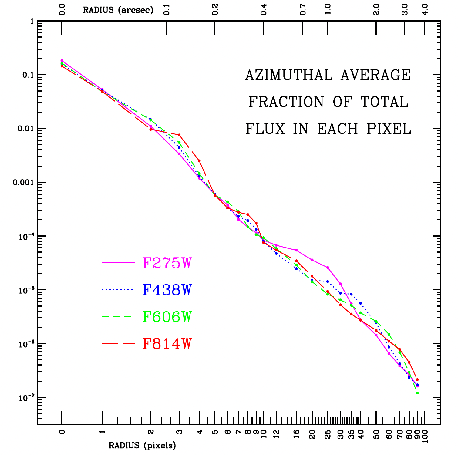
Figure 6.14 plots the azimuthally-averaged model OTA+WFC3 PSF at four different UVIS wavelengths, indicating the fractional PSF flux per pixel at radii from 1 pixel to 4 arcsec.
Figure 6.14: Azimuthally averaged mean WFC3/UVIS PSF in F275W, F438W, F606W, and F814W.
6.6.2 Encircled Energy
The encircled energy is the fraction of the total light from a point source that is contained within a circular aperture of a given radius. Figure 6.15 shows the model PSF encircled energy for 200, 400, and 800 nm. UVIS 1 empirical encircled energy fractions for 10 select aperture radii are given in Table 6.8 (see WFC3 ISR 2016-03 and WFC3 ISR 2022-02 for more details). The WFC3 UVIS Encircled Energy webpage provides the encircled energy curves for both CCDs at 51 total aperture radii as downloadable files. While EE tables have been computed to large radii from deep images of the UVIS PSFs, we do not recommend extrapolating these tables to small apertures (radius < 10 pixels, or ~0.4 arcsec), where the EE varies with detector position and focus level (WFC3 ISR 2025-05). To reduce errors in absolute photometry to better than ~1%, aperture corrections should be measured from isolated stars in the science data or from PSF cutuouts at a similar detector position and focus.
Figure 6.15: Encircled energy for the WFC3/UVIS channel.
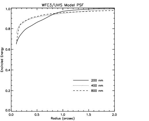
Table 6.8: WFC3/UVIS 1 encircled energy fractions by filter for selected aperture radii (arcsec). To access values for all 51 apertures, see the WFC3 UVIS Encircled Energy webpage. For radii smaller than 0.40 arcsec (10 pixels), the encircled energy fraction can be uncertain up to 1%; for more details, see WFC3 ISR 2025-05.
Filter | Wavelength (Å) | Aperture radius (arcsec) | |||||||||
|---|---|---|---|---|---|---|---|---|---|---|---|
| 0.04 | 0.12 | 0.20 | 0.28 | 0.40 | 0.59 | 0.79 | 0.99 | 1.98 | 6.00 | ||
| F218W | 2228.0 | 0.587 | 0.700 | 0.766 | 0.806 | 0.841 | 0.886 | 0.932 | 0.962 | 0.993 | 1 |
| F225W | 2372.1 | 0.603 | 0.716 | 0.780 | 0.818 | 0.851 | 0.891 | 0.931 | 0.958 | 0.993 | 1 |
| F275W | 2709.7 | 0.173 | 0.673 | 0.793 | 0.837 | 0.865 | 0.893 | 0.921 | 0.945 | 0.983 | 1 |
| F300X | 2820.5 | 0.250 | 0.713 | 0.813 | 0.850 | 0.874 | 0.900 | 0.926 | 0.951 | 0.992 | 1 |
| F280N | 2832.9 | 0.236 | 0.699 | 0.806 | 0.845 | 0.870 | 0.900 | 0.929 | 0.952 | 0.992 | 1 |
| F336W | 3354.5 | 0.203 | 0.666 | 0.816 | 0.863 | 0.890 | 0.911 | 0.929 | 0.946 | 0.991 | 1 |
| F343N | 3435.2 | 0.263 | 0.735 | 0.828 | 0.868 | 0.893 | 0.912 | 0.929 | 0.945 | 0.990 | 1 |
| F373N | 3730.2 | 0.286 | 0.751 | 0.836 | 0.876 | 0.900 | 0.919 | 0.932 | 0.946 | 0.989 | 1 |
| F390M | 3897.2 | 0.275 | 0.745 | 0.831 | 0.870 | 0.898 | 0.917 | 0.932 | 0.945 | 0.989 | 1 |
| F390W | 3923.7 | 0.265 | 0.740 | 0.833 | 0.873 | 0.900 | 0.919 | 0.933 | 0.946 | 0.989 | 1 |
| F395N | 3955.2 | 0.266 | 0.743 | 0.832 | 0.872 | 0.899 | 0.918 | 0.931 | 0.944 | 0.989 | 1 |
| F410M | 4109.0 | 0.152 | 0.646 | 0.823 | 0.869 | 0.901 | 0.922 | 0.934 | 0.946 | 0.988 | 1 |
| F438W | 4326.2 | 0.265 | 0.746 | 0.838 | 0.878 | 0.906 | 0.926 | 0.937 | 0.948 | 0.987 | 1 |
| F467M | 4682.6 | 0.270 | 0.756 | 0.840 | 0.878 | 0.910 | 0.931 | 0.941 | 0.950 | 0.986 | 1 |
| F469N | 4688.1 | 0.267 | 0.747 | 0.835 | 0.874 | 0.906 | 0.928 | 0.939 | 0.949 | 0.986 | 1 |
| F475W | 4773.1 | 0.260 | 0.746 | 0.840 | 0.879 | 0.908 | 0.929 | 0.940 | 0.950 | 0.985 | 1 |
| F487N | 4871.4 | 0.158 | 0.650 | 0.831 | 0.876 | 0.908 | 0.930 | 0.942 | 0.950 | 0.985 | 1 |
| F475X | 4940.7 | 0.192 | 0.671 | 0.805 | 0.845 | 0.908 | 0.903 | 0.927 | 0.946 | 0.985 | 1 |
| F200LP | 4971.9 | 0.241 | 0.738 | 0.840 | 0.879 | 0.908 | 0.929 | 0.940 | 0.950 | 0.985 | 1 |
| F502N | 5009.6 | 0.278 | 0.760 | 0.845 | 0.882 | 0.912 | 0.933 | 0.944 | 0.951 | 0.984 | 1 |
| F555W | 5308.4 | 0.259 | 0.745 | 0.842 | 0.881 | 0.911 | 0.933 | 0.944 | 0.952 | 0.983 | 1 |
| F547M | 5447.5 | 0.248 | 0.745 | 0.842 | 0.880 | 0.911 | 0.934 | 0.946 | 0.953 | 0.982 | 1 |
| F350LP | 5873.9 | 0.237 | 0.725 | 0.834 | 0.873 | 0.904 | 0.926 | 0.939 | 0.949 | 0.980 | 1 |
| F606W | 5889.2 | 0.257 | 0.742 | 0.842 | 0.878 | 0.910 | 0.934 | 0.946 | 0.953 | 0.980 | 1 |
| F621M | 6218.9 | 0.266 | 0.747 | 0.845 | 0.881 | 0.910 | 0.936 | 0.948 | 0.955 | 0.979 | 1 |
| F625W | 6242.6 | 0.242 | 0.730 | 0.841 | 0.878 | 0.909 | 0.934 | 0.947 | 0.954 | 0.979 | 1 |
| F631N | 6304.3 | 0.271 | 0.743 | 0.842 | 0.877 | 0.906 | 0.933 | 0.946 | 0.954 | 0.979 | 1 |
| F645N | 6453.6 | 0.275 | 0.747 | 0.847 | 0.881 | 0.909 | 0.936 | 0.947 | 0.955 | 0.978 | 1 |
| F656N | 6561.4 | 0.271 | 0.740 | 0.844 | 0.877 | 0.908 | 0.935 | 0.948 | 0.957 | 0.978 | 1 |
| F657N | 6566.6 | 0.270 | 0.743 | 0.844 | 0.876 | 0.905 | 0.934 | 0.947 | 0.955 | 0.978 | 1 |
| F658N | 6584.0 | 0.271 | 0.734 | 0.839 | 0.873 | 0.903 | 0.930 | 0.945 | 0.954 | 0.978 | 1 |
| F665N | 6655.9 | 0.269 | 0.738 | 0.843 | 0.876 | 0.906 | 0.935 | 0.948 | 0.956 | 0.978 | 1 |
| F673N | 6765.9 | 0.150 | 0.634 | 0.825 | 0.870 | 0.903 | 0.931 | 0.943 | 0.953 | 0.977 | 1 |
| F689M | 6876.8 | 0.144 | 0.634 | 0.828 | 0.872 | 0.905 | 0.935 | 0.948 | 0.956 | 0.977 | 1 |
| F680N | 6877.6 | 0.260 | 0.729 | 0.843 | 0.874 | 0.905 | 0.933 | 0.947 | 0.954 | 0.977 | 1 |
| F600LP | 7468.1 | 0.238 | 0.716 | 0.842 | 0.874 | 0.906 | 0.933 | 0.947 | 0.955 | 0.976 | 1 |
| F763M | 7614.4 | 0.268 | 0.715 | 0.842 | 0.870 | 0.904 | 0.932 | 0.947 | 0.956 | 0.976 | 1 |
| F775W | 7651.4 | 0.261 | 0.708 | 0.842 | 0.870 | 0.904 | 0.932 | 0.945 | 0.954 | 0.976 | 1 |
| F814W | 8039.1 | 0.239 | 0.686 | 0.836 | 0.868 | 0.902 | 0.929 | 0.943 | 0.953 | 0.975 | 1 |
| F845M | 8439.1 | 0.239 | 0.686 | 0.836 | 0.868 | 0.902 | 0.929 | 0.943 | 0.953 | 0.975 | 1 |
| F850LP | 9176.1 | 0.239 | 0.686 | 0.836 | 0.868 | 0.902 | 0.929 | 0.943 | 0.953 | 0.975 | 1 |
| F953N | 9530.6 | 0.239 | 0.686 | 0.836 | 0.868 | 0.902 | 0.929 | 0.943 | 0.953 | 0.975 | 1 |
6.6.3 Other PSF Behavior and Characteristics
Temporal Dependence of the PSF: HST Breathing
Short term variations in the focus of HST affect all of the data obtained from all of the instruments on HST. A variety of terms, "OTA breathing", "HST breathing", "focus breathing", or simply "breathing" all refer to the same physical behavior. These focus changes are attributed to the contraction/expansion of the OTA due to thermal variations during an orbital period. Thermally-induced HST focus variations also depend on the thermal history of the telescope. For example, after a telescope slew, the telescope temperature variation exhibits the regular orbital component plus a component associated with the change in telescope attitude. The focus changes due to telescope attitude are complicated functions of Sun angle and telescope roll. More information and models can be found on the HST Focus and Pointing webpage.
For WFC3, breathing induces small temporal variations in the UVIS PSF (WFC3 ISR 2012-14). The variations of the UVIS PSF FWHM due to breathing are expected to be as large as 8% at 200 nm, 3% at 400 nm and 0.3% at 800 nm, on typical time scales of one orbit. Some variation over the field of the PSF response to breathing is also expected, since the detector surface is not perfectly matched to the focal surface, and the optical design includes some field-dependent aberration. This field dependence has been analyzed using observations of a globular cluster with filter F606W (WFC3 ISR 2013-11) and deep observations of an isolated star with filter F275W (WFC3 ISR 2013-13). PSFs near the A amplifier on UVIS1 are noticeably elongated by astigmatism. The variation in the asymmetry of PSFs as a function of focus near this amplifier is being explored as a means of measuring breathing and long term focus changes on the UVIS detector (WFC3 ISR 2015-08; WFC3 ISR 2018-14).
Fine guidance jitter can have an impact on the PSF. Historically, HST's jitter has been quite stable at ~ 5 mas. With three functioning gyros, typical variations about this jitter have a negligible contribution to the PSF compared to other known variations (ie. with focus or with location on the detector). As discussed in WFC3 ISR 2025-07, the F606W PSF typically receives 17% of its flux in the central pixel, but this can vary from 15% to 21% depending the location of the star on the detector due to optical effects and variations in the thickness of the CCD. The 17% quoted above is for nominal focus, however, the telescope focus can vary due to HST's thermal history (breathing) and this can lower this fraction to 14%, even in normal operations.
Reduced gyro mode (RGM) with two guide-stars has a marginal effect on guiding, but when a single guide-star is used (1GS/RGM), the orientation of the telescope is under control of the gyros and this can lead to drift of ~ 0.2 pixel over the course of an orbit. This can reduce the central pixel flux from 17% to ~ 15%. These PSF variations are small enough that they do not affect most programs, but programs requiring precise PSFs can mitigate these effects by constructing perturbed PSF models.
Pixel Response Function
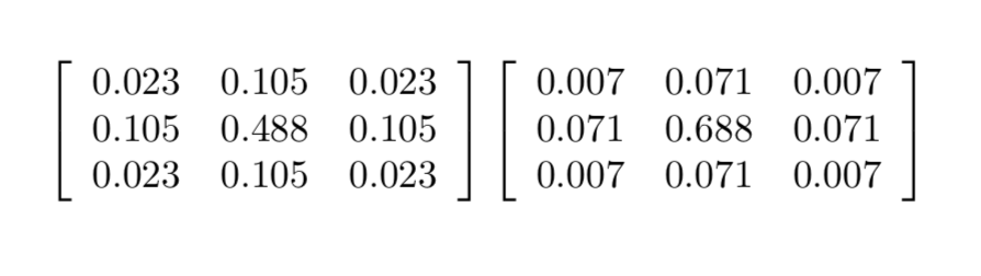
The point-spread function (PSF) is the distribution of light from a point source as spread over a number of pixels. Even with a very compact optical PSF, however, charge diffusion, or migration of charge from one pixel into adjacent neighbor pixels, can degrade the sharpness of a CCD PSF. The effect is usually described in terms of the pixel response function (PRF), which maps the response of the detector to light from a hypothetical very sharp PSF whose light all falls within an individual pixel. Observations using the integrated WFC3 instrument along with optical stimulus point-sources provided empirical PSFs for comparison with, and to provide constraints for, the models. Those models, which included an independent assessment of the low-order wavefront error, the pupil mask, and a reasonable estimate of the detector PRF, yield good agreement with the observed instrumental encircled-energy curves. The resulting best empirical fit to the pixel response convolution kernel is shown in Figure 6.16.
Figure 6.16: CCD Pixel Response functions at 250 nm (left) and 800 nm (right).
PSF Characteristics
The PSF of the UVIS channel was assessed during SMOV in 2009. As part of this assessment, exposures of a field containing unsaturated data (highlighting the bright PSF core) were combined with highly saturated data (emphasizing the faint PSF wings). The results are illustrated in Figure 6.17, which shows the select portions of the composite image with a logarithmic stretch. No geometric distortion correction has been applied, so the images appear elongated along the diagonal, due to the 21 degree tilt of the detector to the chief ray. Although the target was chosen to be isolated, a number of field galaxies appear in the F625W image (right) but are absent in the F275W image; these galaxies are also seen in the IR channel images of the same target (Figure 7.6). Some detector artifacts, including warm pixels and imperfectly removed cosmic ray hits are evident.
Figure 6.17: High dynamic range composite UVIS star images through F275W (left) and F625W (right) subtending ~20 arcsec on each side at different locations in the field.
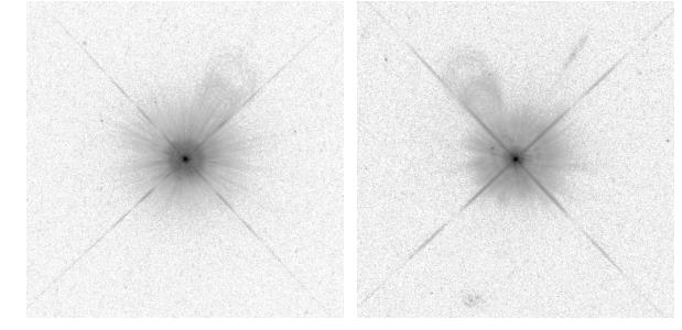
No distortion correction has been applied. Stretch is logarithmic from 1 to 106 e–/pixel. (See text for description of "ghost" artifacts.)
Also evident is a filter ghost, due to reflections between the surfaces of the F625W filter (right). In multi-substrate filters (a stack of two or more substrates bonded or laminated together with a layer of optical adhesive) filter ghosts appear as faint, point-like features, such as the ghost at PA ~65 degrees, radius 1.6 arcsec, in the F625W image, which contains much less than 0.1% of the stellar flux. In single-substrate or air-gap filters (the latter consisting of two substrates joined via thin spacers), filter ghosts appear as small extended shapes (typically rings), closer to the PSF centers than the window ghosts. For the F275W image in Figure 6.13 the filter ghost level is <0.1% and is not obvious. A small number of filters exhibit brighter ghosts; these are discussed in detail in Section 6.5.3 and are tabulated in Table 6.6.
A searchable database of WFC3 PSFs (over 57 million as of 2025, and growing) is publicly available through MAST (WFC3 ISR 2021-12). For more details, see the WFC3 PSF Search webpage.
6.6.4 Super-sampled PSF Models
The PSF that we see exhibited in the image pixels is the combination of many factors: the telescope optics, the filter throughput, integration over the pixel-response function, etc. It is extremely hard to model all of these individual effects accurately, but fortunately that is not necessary. Anderson & King (2000 PASP 112 1360) showed that it is sufficient to model the net PSF, which they call the "effective" PSF. Their initial model was constructed for WFPC2, but since then accurate models have been constructed for a variety of HST instruments and filters.
Their model for the PSF is purely empirical and based on the fundamental question to answer: if a star is centered at location (x,y) on a detector, what fraction of its light will be recorded by pixel [i,j]? The "effective" PSF thus specifies what fraction of a star's light will land in a pixel that is offset by (delta x, delta y) from the center of the star. As such, the effective PSF is simply a two-dimensional function Psi (delta x, delta y) that returns a number between 0.0 and 1.0.
It makes sense that this "effective" PSF function must be smooth and continuous, since moving a star around the detector would result in a continuous variation of recorded flux in each pixel. That said, if the detector is under-sampled, then the "effective" PSF can have sharp variations.
The basis for the PSF model is a simple tabulation of the value of the effective PSF at an array of (delta x, delta y) offsets. This array is spaced by 0.25 flt image pixels, so that it can represent all the structure in WFC3's under-sampled pixels. The PSF model thus consists of an array of 101 x 101 grid points that describe the behavior of the PSF out to a radius of 12.5 pixels. The PSFs are normalized to have a total flux of 1.0 within 10.0 pixels for WFC3/UVIS and within 5.5 pixels for WFC3/IR. Bi-cubic spline interpolation is adequate to interpolate the table to locations between the grid points.
The PSF also changes with location on the detector, so the models provide the PSF at an array of fiducial locations across the detectors. Simple bi-linear interpolation is adequate to provide a complete 101 x 101 PSF model at any given location on the detector. The PSF is thus a four-dimensional function: Psi (delta x, delta y; x, y).
Figure 6.18 shows the array of fiducial points where the WFC3/UVIS PSF is provided for the F606W filter. On the left is a schematic of the detector and on the right the central value of the PSF, which represents the fraction of light from a point source that would land in a pixel if the star is exactly centered on that pixel. The fraction goes from about 16 percent in the upper left corner to over 22 percent in the region of strong fringing in red narrow-band filters (WFC3 ISR 2010-04) in the lower right-middle of the bottom chip.
Figure 6.18: Locations of PSF models on the detector (left) and percentage of flux in the peak pixel for a pixel-centered PSF at each location.
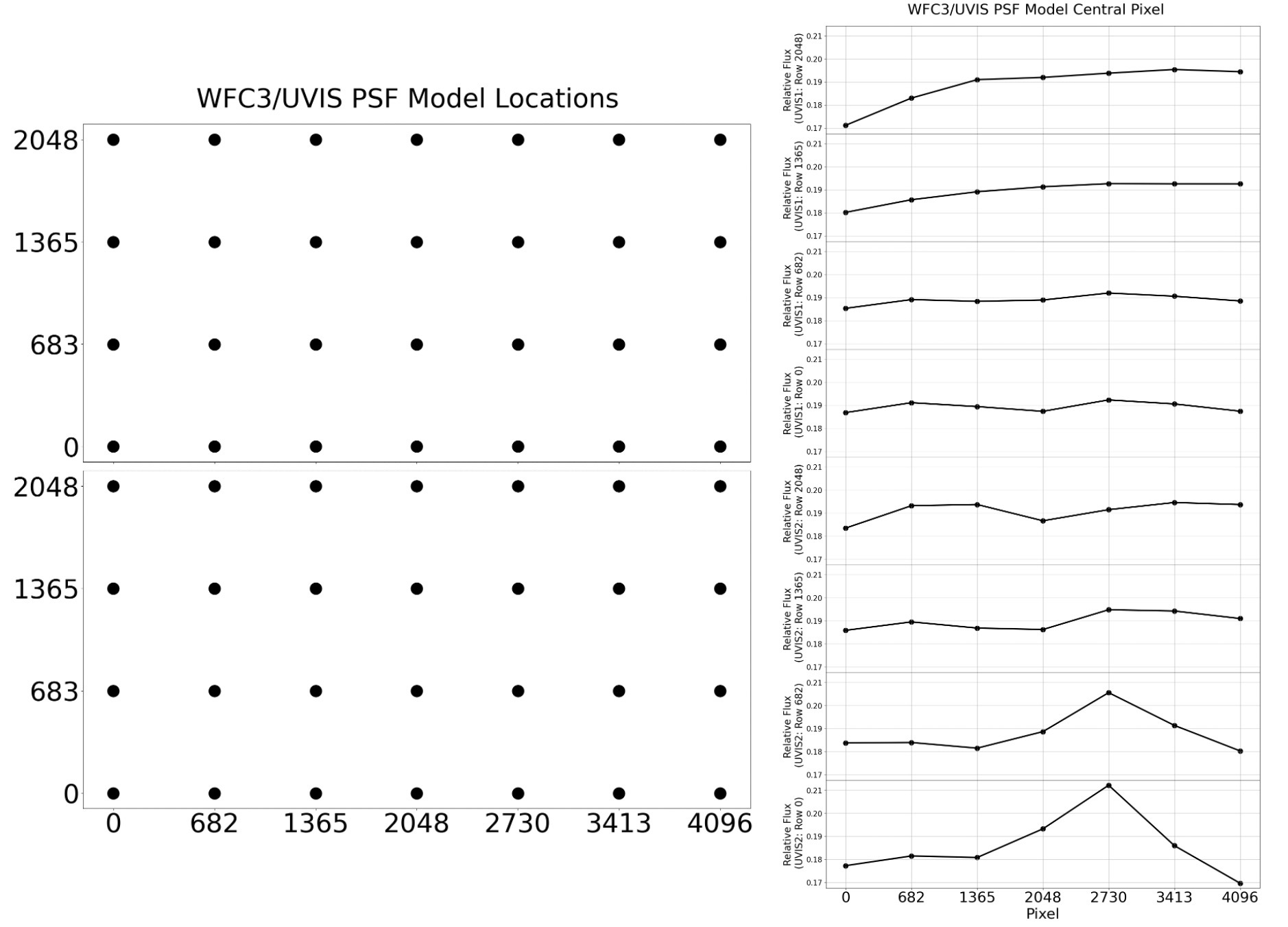
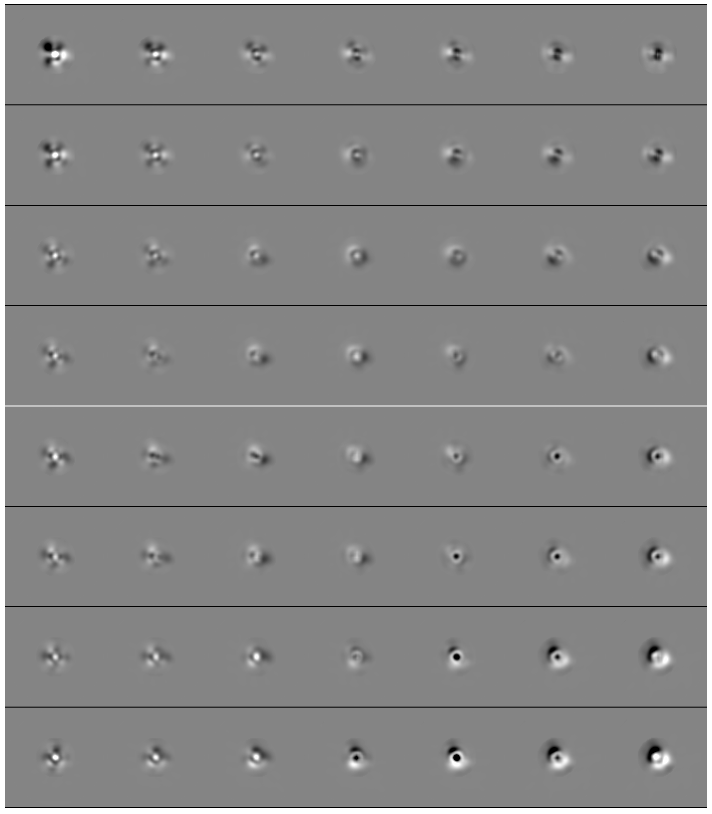
Figure 6.19: Difference between the super-sampled PSF at the locations shown in Figure 6.18 and the average of these PSFs. Black indicates greater than average flux.
Note that the above PSF discussion applies only for un-resampled "flt"-type images (see WFC3 Data Handbook), since these are the images where each pixel can be a direct physical constraint on the scene. The "drz"-type images have been resampled, such that each pixel represents some combination of input pixels from one or multiple exposures. Such images are not well suited to high-precision PSF analysis. There are several challenges, however, in working in the "flt" frame. The first is that the images are generally under-sampled, such that each exposure is not a full representation of the astronomical scene. One generally must combine several dithered "flt"-type images to fully constrain the scene delivered to the telescope. The second challenge is that the "flt" images are severely distorted, and it is non-trivial to collect these constraints on the scene and analyze them together. For these reasons, even if a user does have access to a perfectly accurate PSF for a given exposure, it still requires considerable expertise to use it for analysis.
The instrument team, being aware of these challenges, has been working to provide PSF-related tools for users. Spatially variable, super-sampled models of the PSF can be found on the WFC3 PSF webpage, which contains additional resources relating to PSFs. Recently, a software routine that makes use of the PSFs to measure stars in HST images was released. This routine is named hst1pass, and WFC3 ISR 2022-05 describes how it can be downloaded and run. In 2024 the team added a Jupyter notebook for generating PSF models, also found on the PSF webpage.
In an effort to supplement these super-sampled model PSFs, the WFC3 team recently has built a searchable database of over 57 million WFC3 star images (PSFs extracted from science images) from 2009 to 2022. The PSF image library can also be searched using a team-developed Jupyter notebook (see WFC3 ISR 2021-12 and the WFC3 PSF Search webpage for more details). These images of PSFs can then be employed to generate PSFs for users' observations and other science needs.
-
WFC3 Instrument Handbook
- • Acknowledgments
- Chapter 1: Introduction to WFC3
- Chapter 2: WFC3 Instrument Description
- Chapter 3: Choosing the Optimum HST Instrument
- Chapter 4: Designing a Phase I WFC3 Proposal
- Chapter 5: WFC3 Detector Characteristics and Performance
-
Chapter 6: UVIS Imaging with WFC3
- • 6.1 WFC3 UVIS Imaging
- • 6.2 Specifying a UVIS Observation
- • 6.3 UVIS Channel Characteristics
- • 6.4 UVIS Field Geometry
- • 6.5 UVIS Spectral Elements
- • 6.6 UVIS Optical Performance
- • 6.7 UVIS Exposure and Readout
- • 6.8 UVIS Sensitivity
- • 6.9 Charge Transfer Efficiency
- • 6.10 Other Considerations for UVIS Imaging
- • 6.11 UVIS Observing Strategies
- Chapter 7: IR Imaging with WFC3
- Chapter 8: Slitless Spectroscopy with WFC3
-
Chapter 9: WFC3 Exposure-Time Calculation
- • 9.1 Overview
- • 9.2 The WFC3 Exposure Time Calculator - ETC
- • 9.3 Calculating Sensitivities from Tabulated Data
- • 9.4 Count Rates: Imaging
- • 9.5 Count Rates: Slitless Spectroscopy
- • 9.6 Estimating Exposure Times
- • 9.7 Sky Background
- • 9.8 Interstellar Extinction
- • 9.9 Exposure-Time Calculation Examples
- Chapter 10: Overheads and Orbit Time Determinations
-
Appendix A: WFC3 Filter Throughputs
- • A.1 Introduction
-
A.2 Throughputs and Signal-to-Noise Ratio Data
- • UVIS F200LP
- • UVIS F218W
- • UVIS F225W
- • UVIS F275W
- • UVIS F280N
- • UVIS F300X
- • UVIS F336W
- • UVIS F343N
- • UVIS F350LP
- • UVIS F373N
- • UVIS F390M
- • UVIS F390W
- • UVIS F395N
- • UVIS F410M
- • UVIS F438W
- • UVIS F467M
- • UVIS F469N
- • UVIS F475W
- • UVIS F475X
- • UVIS F487N
- • UVIS F502N
- • UVIS F547M
- • UVIS F555W
- • UVIS F600LP
- • UVIS F606W
- • UVIS F621M
- • UVIS F625W
- • UVIS F631N
- • UVIS F645N
- • UVIS F656N
- • UVIS F657N
- • UVIS F658N
- • UVIS F665N
- • UVIS F673N
- • UVIS F680N
- • UVIS F689M
- • UVIS F763M
- • UVIS F775W
- • UVIS F814W
- • UVIS F845M
- • UVIS F850LP
- • UVIS F953N
- • UVIS FQ232N
- • UVIS FQ243N
- • UVIS FQ378N
- • UVIS FQ387N
- • UVIS FQ422M
- • UVIS FQ436N
- • UVIS FQ437N
- • UVIS FQ492N
- • UVIS FQ508N
- • UVIS FQ575N
- • UVIS FQ619N
- • UVIS FQ634N
- • UVIS FQ672N
- • UVIS FQ674N
- • UVIS FQ727N
- • UVIS FQ750N
- • UVIS FQ889N
- • UVIS FQ906N
- • UVIS FQ924N
- • UVIS FQ937N
- • IR F098M
- • IR F105W
- • IR F110W
- • IR F125W
- • IR F126N
- • IR F127M
- • IR F128N
- • IR F130N
- • IR F132N
- • IR F139M
- • IR F140W
- • IR F153M
- • IR F160W
- • IR F164N
- • IR F167N
- Appendix B: Geometric Distortion
- Appendix C: Dithering and Mosaicking
- Appendix D: Bright-Object Constraints and Image Persistence
-
Appendix E: Reduction and Calibration of WFC3 Data
- • E.1 Overview
- • E.2 The STScI Reduction and Calibration Pipeline
- • E.3 The SMOV Calibration Plan
- • E.4 The Cycle 17 Calibration Plan
- • E.5 The Cycle 18 Calibration Plan
- • E.6 The Cycle 19 Calibration Plan
- • E.7 The Cycle 20 Calibration Plan
- • E.8 The Cycle 21 Calibration Plan
- • E.9 The Cycle 22 Calibration Plan
- • E.10 The Cycle 23 Calibration Plan
- • E.11 The Cycle 24 Calibration Plan
- • E.12 The Cycle 25 Calibration Plan
- • E.13 The Cycle 26 Calibration Plan
- • E.14 The Cycle 27 Calibration Plan
- • E.15 The Cycle 28 Calibration Plan
- • E.16 The Cycle 29 Calibration Plan
- • E.17 The Cycle 30 Calibration Plan
- • E.18 The Cycle 31 Calibration Plan
- • E.19 The Cycle 32 Calibration Plan
- • E.20 The Cycle 33 Calibration Plan
- • Glossary