7.6 IR Optical Performance
Following WFC3's alignment to the OTA (WFC3 ISR 2009-46), a series of observations through a variety of filters were obtained to demonstrate the instrument's optical performance. The WFC3/IR channel met or exceeded all image quality expectations. The following subsections summarize the measured flight optical performance for the IR channel, as described by its point-spread function (PSF), i.e., the spatial distribution of the flux in an image of a point source. The results shown were produced using an optical model which was adjusted and correlated to the PSFs measured on-orbit and represent mean values averaged over the field (WFC3 ISR 2009-37). This PSF model includes the pupil geometry, including the cold stop, residual aberration, the mid-frequency wavefront error of the OTA, the effect of the detector inter-pixel capacitive cross-talk, and first-order geometric distortion.
HST is designed to use two guide stars in the fine-guidance sensors (FGSs) to maintain its pointing and tracking during exposures. However, HST is also able to track using only a single GS in conjunction with a gyro. The pointing quality achieved in this latter case is equivalent to two GSs for exposures < 500 sec. Over the course a full orbit (~ 2500 sec), the drift is typically < 0.1 IR pixel but can range up to 0.15 pix; the impact on IR imaging is smaller than UVIS imaging (see Section 6.6). Such a drift should have a minimal impact on most science programs, since the variation in the PSF caused by drift is smaller than the PSF variations with focus and with location on the detector. For further information, see WFC3 ISR 2025-07.
7.6.1 PSF Width and Sharpness
The IR channel PSFs are well approximated by Gaussian profiles (before pixelation). As was discussed in more detail for the UVIS channel in Section 6.6.1, the PSFs can usefully be characterized by their FWHM or their sharpness, effectively the reciprocal of the number of pixels occupied by a point source (as defined in Section 6.6.1). Table 7.5 lists the FWHM of the model PSF core (before pixelation) in units of pixel and arcsec and the sharpness parameter for 10 wavelengths. The sharpness range shown for each wavelength indicates the values for the PSF centered on the pixel corners and center. The monotonic increase in FWHM and decrease in sharpness with wavelength is due to diffraction.
Table 7.5: WFC3/IR PSF FWHM (before pixelation, in units of pixels and arcseconds), and sharpness, vs. wavelength. (Note that attempts to measure the FWHM by fitting functions to the pixelated PSF will generally yield larger values.)
Wavelength | FWHM | FWHM | Sharpness |
800 | 0.971 | 0.124 | 0.127–0.197 |
900 | 0.986 | 0.126 | 0.118–0.182 |
1000 | 1.001 | 0.128 | 0.109–0.169 |
1100 | 1.019 | 0.130 | 0.100–0.156 |
1200 | 1.040 | 0.133 | 0.093–0.144 |
1300 | 1.067 | 0.137 | 0.087–0.132 |
1400 | 1.100 | 0.141 | 0.083–0.121 |
1500 | 1.136 | 0.145 | 0.080–0.112 |
1600 | 1.176 | 0.151 | 0.077–0.102 |
1700 | 1.219 | 0.156 | 0.074–0.093 |
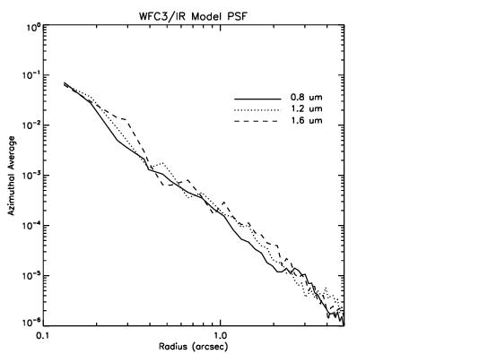
Figure 7.5 plots the azimuthally-averaged model OTA+WFC3 PSF at three different IR wavelengths., indicating the fractional PSF flux per pixel at radii from 1 pixel to 5 arcsec.
Figure 7.5: Azimuthally averaged WFC3/IR PSF.
7.6.2 Encircled Energy
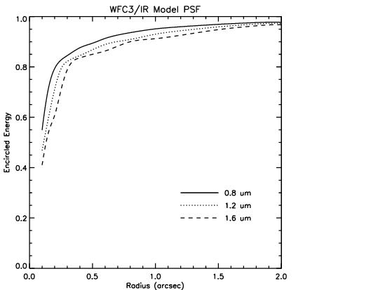
As described in more detail in Section 6.6.2 for the UVIS channel, encircled energy, the fraction of light contained in a circular aperture is one useful way of characterizing well-behaved profiles. Encircled energy profiles for the IR channel model PSF at three representative wavelengths are plotted in Figure 7.6. Empirical encircled energy values for 11 select aperture radii are presented in Table 7.6 (see WFC3 ISR 2009-37 for more details). The WFC3 IR Encircled Energy webpage provides the encircled energy curves for 19 total aperture radii as a downloadable file.
Figure 7.6: Encircled Energy for the WFC3/IR channel.
| Filter | Wavelength (Å) | Aperture (arcsec) | ||||||||||
|---|---|---|---|---|---|---|---|---|---|---|---|---|
| 0.13 | 0.26 | 0.39 | 0.52 | 0.65 | 0.78 | 0.91 | 1.0 | 1.3 | 2.0 | 6.0 | ||
| F098M | 9865 | 0.596 | 0.818 | 0.857 | 0.887 | 0.905 | 0.922 | 0.934 | 0.943 | 0.956 | 0.974 | 1 |
| F105W | 10551 | 0.577 | 0.811 | 0.852 | 0.882 | 0.901 | 0.917 | 0.929 | 0.939 | 0.953 | 0.973 | 1 |
| F110W | 11534 | 0.553 | 0.797 | 0.845 | 0.873 | 0.895 | 0.909 | 0.922 | 0.933 | 0.948 | 0.97 | 1 |
| F125W | 12486 | 0.535 | 0.789 | 0.841 | 0.867 | 0.89 | 0.904 | 0.918 | 0.929 | 0.945 | 0.969 | 1 |
| F126N | 12585 | 0.534 | 0.789 | 0.84 | 0.867 | 0.89 | 0.904 | 0.917 | 0.929 | 0.944 | 0.969 | 1 |
| F127M | 12740 | 0.531 | 0.787 | 0.84 | 0.865 | 0.89 | 0.903 | 0.916 | 0.929 | 0.944 | 0.968 | 1 |
| F128N | 12832 | 0.529 | 0.786 | 0.839 | 0.865 | 0.889 | 0.902 | 0.916 | 0.928 | 0.943 | 0.968 | 1 |
| F130N | 13006 | 0.526 | 0.784 | 0.838 | 0.863 | 0.888 | 0.901 | 0.915 | 0.927 | 0.942 | 0.968 | 1 |
| F132N | 13188 | 0.523 | 0.78 | 0.838 | 0.862 | 0.887 | 0.9 | 0.914 | 0.926 | 0.942 | 0.967 | 1 |
| F139M | 13838 | 0.513 | 0.769 | 0.836 | 0.858 | 0.882 | 0.898 | 0.912 | 0.923 | 0.939 | 0.966 | 1 |
| F140W | 13923 | 0.512 | 0.764 | 0.837 | 0.86 | 0.882 | 0.9 | 0.912 | 0.923 | 0.94 | 0.967 | 1 |
| F153M | 15322 | 0.496 | 0.74 | 0.835 | 0.856 | 0.876 | 0.899 | 0.909 | 0.918 | 0.937 | 0.967 | 1 |
| F160W | 15369 | 0.494 | 0.736 | 0.833 | 0.855 | 0.875 | 0.897 | 0.908 | 0.918 | 0.935 | 0.966 | 1 |
| F164N | 16404 | 0.483 | 0.713 | 0.829 | 0.852 | 0.87 | 0.894 | 0.905 | 0.914 | 0.932 | 0.963 | 1 |
| F167N | 16642 | 0.48 | 0.706 | 0.828 | 0.851 | 0.869 | 0.893 | 0.904 | 0.913 | 0.931 | 0.962 | 1 |
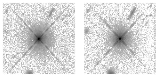
During initial on-orbit tests in SMOV, high-dynamic-range isolated star images were obtained through several filters (WFC3 ISR 2009-37). These are shown with a logarithmic stretch in Figure 7.7. The images appear slightly elongated vertically, due to the 24 degree tilt of the detector to the chief ray and the fact that a distortion correction has not been applied. Although the target was chosen to be isolated, a number of field galaxies appear in both the F098M and the F160W filter images; these are also seen in long wavelength UVIS channel images of the same target (Figure 6.13). Some detector artifacts, including cold and warm pixels and imperfectly removed cosmic ray hits are evident.
Figure 7.7: High dynamic range WFC3/IR star images through F098M (left) and F160W (right) subtending ~20 arcsec on each side near field center. No distortion correction has been applied. Stretch is logarithmic from 10–3 to 103 e– sec–1 pixel–1. Faint galaxies appear in the background.
7.6.3 Other PSF Behavior and Characteristics
Temporal Dependence of the PSF: HST Breathing
All HST observations are affected to some extent by short-term focus variations (“breathing”), which arise from the changing thermal environment of HST (See Section 6.6.3). For the IR channel, breathing is expected to produce variations of ~0.3% and less than 0.1% in the FWHM of the PSF of WFC3/IR at 700 nm and at wavelengths longer than 1100 nm, respectively, on typical time scales of one orbit.
Intra-Pixel Response
The response of a pixel of an IR detector to light from an unresolved source varies with the positioning of the source within the pixel due to low sensitivity at the pixel's edges and dead zones between pixels. For the WFC3/IR flight detector, no measurable intra-pixel sensitivity variation was found during ground testing (WFC3 ISR 2008-19) or in-flight testing (WFC3 ISR 2011-19). For NICMOS, the intra-pixel sensitivity was found to be an important effect: it varied by as much as 40% (peak to valley). The WFC3 small pixel size (18 µm vs. NICMOS's 40 µm) and the much higher WFC3/IR detector temperature compared to NICMOS are probably responsible for this improvement.
Inter-Pixel Capacitance
The small pixel size, relative to that in NICMOS, increases the relevance of capacitive coupling between nearby pixels (Brown et. al., 2006, PASP, 118, 1443; Moore et. al., 2006, Opt. Eng., 076402). It affects the gain measurements and the PSF. The easiest method of estimating the inter-pixel capacitance is to measure the ratio of DNs in pixels adjacent to a “hot” (high-dark-current) pixel to the DNs in the hot pixel. In the WFC3 IR detector, on the order of 5% of electrons may leak to the adjacent pixels. WFC3 ISR 2008-26 describes a method for correcting inter-pixel capacitance using Fourier deconvolution, and demonstrates its effectiveness on WFC3/IR ground-testing data. WFC3 ISR 2011-10 provides an improved deconvolution kernel with distinct values for each of the 8 pixels surrounding the central pixel.
7.6.4 Super-sampled PSF Models
The concept of empirical net (“effective”) models of PSFs is introduced in Section 6.6.4. The WFC3/IR PSF has recently been modeled in WFC3 ISR 2016-12 for five commonly used filters (F105W, F110W, F125W, F140W, and F160W); these models are available to download on the WFC3 PSF webpage. Other filters are expected to be added in the future.
Figure 7.8 shows a log image of the F105W PSF in super-sampled (4x) pixels. The WFC3/IR PSF is extremely under-sampled by the detector pixels: over 40 percent of a star's flux will land in its central pixel if the star is centered on that pixel. Only 4 percent will fall in the directly adjacent pixels. Even with this extreme under-sampling, the 4x super-sampled grid-base model is easily able to represent the PSF.
Figure 7.8: An image of the central WFC3/IR PSF for F105W where the PSF is super-sampled by a factor of 4 relative to the WFC3/IR image pixels.
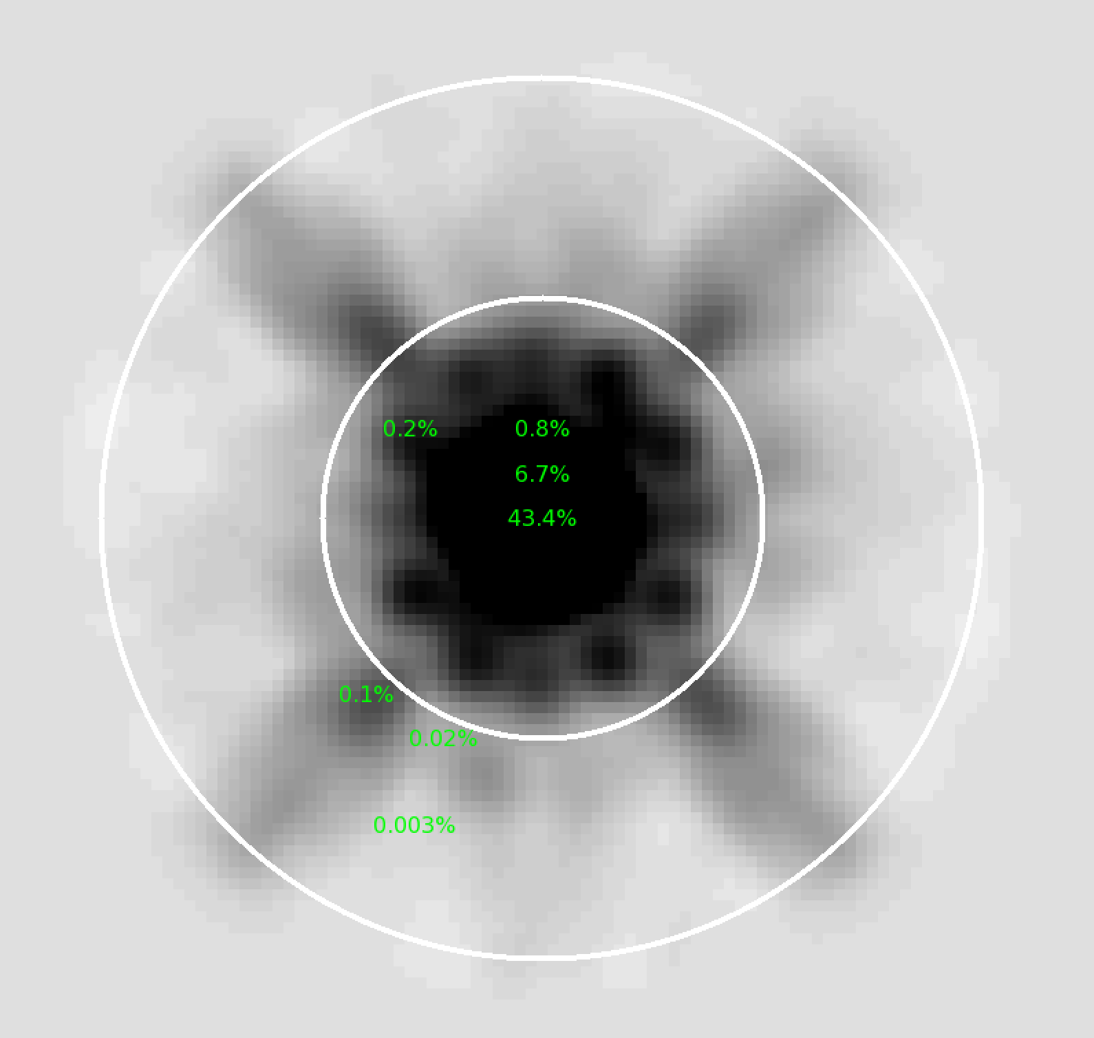
The white circles are drawn at r=5 and r=10 image pixels. The central label (43.4%) shows how much of the star's flux should be received by a pixel if the star happens to be centered on exactly that pixel. The label above it (6.7%) is the fraction of a star's flux which would land in a pixel that is exactly one image-pixel above the center of the star. The 0.8% label is the amount of light which would land in a pixel two up from the center of a star. The other labels show the fraction of light that lands in pixels at various other locations in the PSF: on inner-halo bumps (0.2%), on diffraction spikes at a distance of ~5 image pixels (0.1%), in the outer PSF halo at ~5 image pixels (0.02%) and in the outer halo at ~7.5 image pixels (0.003%).
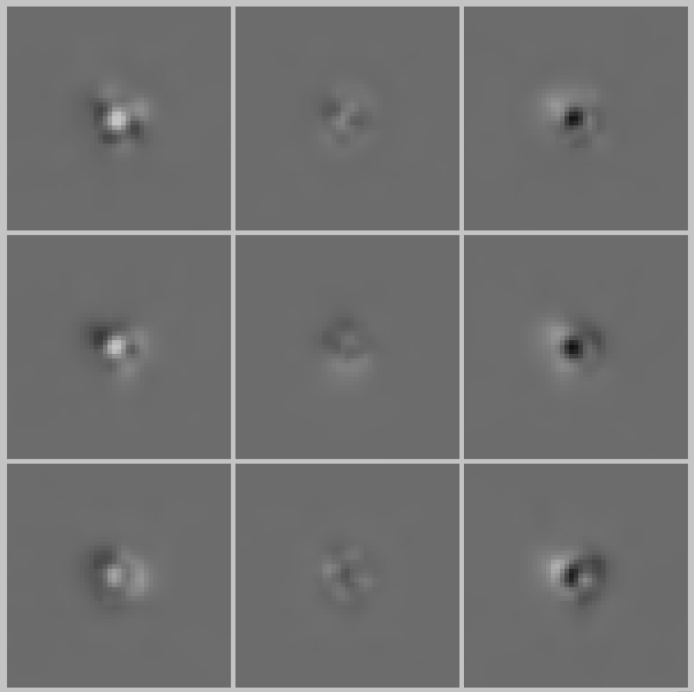
Figure 7.9: For 9 locations on the detector in a 3 × 3 grid, a greyscale image shows the difference between each super-sampled PSF and the average of the PSFs. Dark represents more flux, and light less flux. The largest variation is about 0.04, which is about 10% of the central value of the PSF.
hst1pass, and WFC3 ISR 2022-05 describes how it can be downloaded and run.In an effort to supplement these super-sampled model PSFs, the WFC3 team recently has built a searchable database of over 26 million WFC3/IR extracted star images (PSFs) from 2009 to 2023 (see WFC3 ISR 2021-12 and the WFC3 PSF Search webpage for more details). These images of PSFs can then be employed to generate PSFs that for users' observations and other science needs. The WFC3 team additionally provides a tutorial of how to download these cutouts in the form of a Jupyter notebook.
-
WFC3 Instrument Handbook
- • Acknowledgments
- Chapter 1: Introduction to WFC3
- Chapter 2: WFC3 Instrument Description
- Chapter 3: Choosing the Optimum HST Instrument
- Chapter 4: Designing a Phase I WFC3 Proposal
- Chapter 5: WFC3 Detector Characteristics and Performance
-
Chapter 6: UVIS Imaging with WFC3
- • 6.1 WFC3 UVIS Imaging
- • 6.2 Specifying a UVIS Observation
- • 6.3 UVIS Channel Characteristics
- • 6.4 UVIS Field Geometry
- • 6.5 UVIS Spectral Elements
- • 6.6 UVIS Optical Performance
- • 6.7 UVIS Exposure and Readout
- • 6.8 UVIS Sensitivity
- • 6.9 Charge Transfer Efficiency
- • 6.10 Other Considerations for UVIS Imaging
- • 6.11 UVIS Observing Strategies
- Chapter 7: IR Imaging with WFC3
- Chapter 8: Slitless Spectroscopy with WFC3
-
Chapter 9: WFC3 Exposure-Time Calculation
- • 9.1 Overview
- • 9.2 The WFC3 Exposure Time Calculator - ETC
- • 9.3 Calculating Sensitivities from Tabulated Data
- • 9.4 Count Rates: Imaging
- • 9.5 Count Rates: Slitless Spectroscopy
- • 9.6 Estimating Exposure Times
- • 9.7 Sky Background
- • 9.8 Interstellar Extinction
- • 9.9 Exposure-Time Calculation Examples
- Chapter 10: Overheads and Orbit Time Determinations
-
Appendix A: WFC3 Filter Throughputs
- • A.1 Introduction
-
A.2 Throughputs and Signal-to-Noise Ratio Data
- • UVIS F200LP
- • UVIS F218W
- • UVIS F225W
- • UVIS F275W
- • UVIS F280N
- • UVIS F300X
- • UVIS F336W
- • UVIS F343N
- • UVIS F350LP
- • UVIS F373N
- • UVIS F390M
- • UVIS F390W
- • UVIS F395N
- • UVIS F410M
- • UVIS F438W
- • UVIS F467M
- • UVIS F469N
- • UVIS F475W
- • UVIS F475X
- • UVIS F487N
- • UVIS F502N
- • UVIS F547M
- • UVIS F555W
- • UVIS F600LP
- • UVIS F606W
- • UVIS F621M
- • UVIS F625W
- • UVIS F631N
- • UVIS F645N
- • UVIS F656N
- • UVIS F657N
- • UVIS F658N
- • UVIS F665N
- • UVIS F673N
- • UVIS F680N
- • UVIS F689M
- • UVIS F763M
- • UVIS F775W
- • UVIS F814W
- • UVIS F845M
- • UVIS F850LP
- • UVIS F953N
- • UVIS FQ232N
- • UVIS FQ243N
- • UVIS FQ378N
- • UVIS FQ387N
- • UVIS FQ422M
- • UVIS FQ436N
- • UVIS FQ437N
- • UVIS FQ492N
- • UVIS FQ508N
- • UVIS FQ575N
- • UVIS FQ619N
- • UVIS FQ634N
- • UVIS FQ672N
- • UVIS FQ674N
- • UVIS FQ727N
- • UVIS FQ750N
- • UVIS FQ889N
- • UVIS FQ906N
- • UVIS FQ924N
- • UVIS FQ937N
- • IR F098M
- • IR F105W
- • IR F110W
- • IR F125W
- • IR F126N
- • IR F127M
- • IR F128N
- • IR F130N
- • IR F132N
- • IR F139M
- • IR F140W
- • IR F153M
- • IR F160W
- • IR F164N
- • IR F167N
- Appendix B: Geometric Distortion
- Appendix C: Dithering and Mosaicking
- Appendix D: Bright-Object Constraints and Image Persistence
-
Appendix E: Reduction and Calibration of WFC3 Data
- • E.1 Overview
- • E.2 The STScI Reduction and Calibration Pipeline
- • E.3 The SMOV Calibration Plan
- • E.4 The Cycle 17 Calibration Plan
- • E.5 The Cycle 18 Calibration Plan
- • E.6 The Cycle 19 Calibration Plan
- • E.7 The Cycle 20 Calibration Plan
- • E.8 The Cycle 21 Calibration Plan
- • E.9 The Cycle 22 Calibration Plan
- • E.10 The Cycle 23 Calibration Plan
- • E.11 The Cycle 24 Calibration Plan
- • E.12 The Cycle 25 Calibration Plan
- • E.13 The Cycle 26 Calibration Plan
- • E.14 The Cycle 27 Calibration Plan
- • E.15 The Cycle 28 Calibration Plan
- • E.16 The Cycle 29 Calibration Plan
- • E.17 The Cycle 30 Calibration Plan
- • E.18 The Cycle 31 Calibration Plan
- • E.19 The Cycle 32 Calibration Plan
- • E.20 The Cycle 33 Calibration Plan
- • Glossary