7.10 IR Observing Strategies

7.10.1 Dithering Strategies

For imaging programs, STScI generally recommends that observers employ dithering patterns. Dithering refers to the procedure of moving the telescope by small angle offsets between individual exposures on a target. The resulting images are subsequently combined in the pipeline or by the observer using software such as AstroDrizzle.

Dithering is used to improve both image quality and resolution. By combining multiple images of a target at slightly different positions on the detector, one can compensate for detector artifacts (blemishes, dead pixels, hot pixels, transient bad pixels, flatfielding errors, and plate-scale irregularities) that may not be completely corrected by application of the calibration reference files. Combining images, whether dithered or not, can also remove any residual cosmic ray flux that has not been well removed by the up-the-ramp fitting procedure used to produce flt images (see Section 7.7.2 and Appendix E). Effective resolution can be improved by combining images made with sub-pixel offsets designed to better sample the PSF which is particularly important for WFC3/IR because the PSF is undersampled by about a factor of 2 (Table 7.5).

Larger offsets are used to mosaic a region of sky larger than the detector field of view and can also be used for “chopping” to sample the thermal background. While "chopping" was recommended for NICMOS exposures at wavelengths longer than 1.7 microns, where the telescope thermal background becomes dominant, the thermal background is not a problem for WFC3/IR. In WFC3, all offsets must be accomplished by moving the telescope (in NICMOS it was also possible to move the Field Offset Mirror).

Dithers must be contained within a diameter ~130 arcsec or less (depending on the availability of guide stars in the region) to use the same guide stars for all exposures. The rms pointing repeatability is significantly less accurate if different guide stars are used for some exposures (see Appendix B of the DrizzlePac Handbook). Mosaic steps and small dither steps are often combined to increase the sky coverage while also increasing resolution and removing artifacts. Section 6.11.1 provides a discussion of the effect of geometric distortion on PSF sampling for mosaic steps.

The set of Pattern Parameters in the observing proposal provides a convenient means for specifying the desired pattern of offsets. The pre-defined mosaic and dither patterns that have been implemented in APT to meet many of the needs outlined above are described in detail in the Phase II Proposal Instructions. The WFC3 patterns in effect in APT at the time of publication of this Handbook are summarized in Appendix C. Observers can define their own APT patterns to tailor them to the amount of allocated observing time and the desired science goals of the program. Alternatively, they can use POS TARGs to implement dither steps (Section 7.4.3). WFC3 ISR 2016-14 provides compact patterns with up to 9 steps (in the form of POS TARGs) designed to preserve sub-pixel sampling as much as possible over the face of the detector, given the scale changes introduced by geometric distortion. Observers should note that thermally-driven drift of the image on the detector, occasionally larger than 0.15 pixels in two orbits, will limit the accuracy of execution of dither patterns (WFC3 ISR 2009-32). Additional information on dither strategies can be found in WFC3 ISR 2010-09, which provides a decision tree for selecting patterns and combining them with sub-patterns. 

7.10.2 Parallel Observations

Parallel observations, i.e., the simultaneous use of WFC3 with one or more other HST instruments, are the same for the IR channel as for the UVIS channel, previously described in Section 6.11.2. Note that there are new patterns available to optimize dither patterns for proposals using WFC3 and ACS simultaneously (WFC3 ISR 2023-05).

7.10.3 Exposure Strategies

Given the variety of requirements of the scientific programs that are being executed with WFC3/IR, it is impossible to establish a single optimum observing strategy. In this section we therefore provide a few examples after guiding the reader through the main constraints that should be taken into account when designing an observation:

• Integrate long enough to be limited by background emission and not read noise. Dark current (~0.05 e^–/s/pixel) is rarely the limiting factor.
• Dither enough so that resolution can be restored to the diffraction limit and bad pixels and cosmic-ray impacts can be removed, while maintaining a homogeneous SNR across the field.
• Dither in large enough steps (> 10 pixels, WFC3 ISR 2019-07) and sequence exposures from low to high S/N when possible to avoid self-persistence.
  
• Use MULTIACCUM ramps with as many reads as possible for readout noise suppression.
  

In this regard, it is useful to consider Table 7.12, which summarizes the total background seen by a pixel, including sky, telescope, and nominal dark current, and the time needed to reach 400 e^–/pixel of accumulated signal, corresponding to 20 e^–/pixel of Poisson-distributed background noise. The latter, higher than the expected readout noise of ~12 electrons after 16 reads, is used here to set the threshold for background-limited performance. The passage from readout-limited performance to background-limited performance can be regarded as the optimal exposure time for that given filter, in the sense that it allows for the largest number of dithered images without significant loss of SNR (for a given total exposure time, i.e., neglecting overheads). For faint sources, the optimal integration time strongly depends on the background (zodiacal, Earth-shine thermal, and dark current) in each filter, ranging from just 220 s for the F110W filter to 2700 s for some of the narrow-band filters.

These constraints put contradictory requirements on the ideal observing strategy. It is clear that given a certain amount of total observing time, the requirement of long integrations for background limited performance is incompatible with a large number of dithering positions. Also, to increase the number of reads within a ramp for readout noise suppression decreases the observing efficiency, with a negative impact on the signal to noise ratio. Because the background seen by each pixel depends on the filter (Section 7.9.5), the optimal compromise must be determined on a case-by-case basis.

The optimal integration time needed to reach background-limited performance (Table 7.12) can be compared with the integration times of the sampling sequences from Table 7.8. Table 7.13 synthesizes the results, showing for each filter which sample sequence most closely matches the optimal integration times for NSAMP=15.

Table 7.12: Background levels  (e–/pix/s) at the WFC3/IR detector. The columns show, from left to right: a) filter name; b) thermal background from the telescope and instrument; c) zodiacal background; d) earth-shine background; e) dark current; f) total background; g) integration time needed to reach background-limited performance, assuming an equivalent readout noise of 20 electrons.

The selection of sample sequence type (RAPID, SPARS, STEP; Section 7.7.3) must take into account the science goals and the restrictions placed on their use. Most observers have found that the SPARS ramps best meet the needs of their programs. Here are some factors to consider when selecting a sample sequence:

• The RAPID ramp is a uniform sequence of short exposures. With its relatively short maximum exposure time, RAPID is suitable for a target consisting of bright objects that would saturate after a few reads in the other sequences. It is not appropriate for background-limited performance.
• SPARS ramps, with their uniform sampling, provide the most robust rejection of cosmic-ray events, and can be trimmed by removing a few of the final reads to fine-tune the integration time with little degradation of the achieved readout noise. Thus they are considered the standard sampling mode.
  
• STEP ramps are preferable where large dynamic range is needed; e.g., for photometry of stellar clusters. These ramps begin with a sequence of four uniform (RAPID) reads and end with a sequence of much longer uniform reads. The transition between the two uniform read rates is provided by a short sequence of logarithmically increasing read times. This design provides for correction of any non-linearities early in the exposure and allows for increased dynamic range for both bright and faint targets.

Finally, the selection of a given sample sequence type should also be made in conjunction with the number of samples (nsamp) that will be used to achieve the desired total exposure time for the observation. Long exposures should in general use a minimum of 5-6 samples in order to allow for reliable CR rejection and to allow for at least a few unsaturated samples of bright targets in the field. For very faint targets in read-noise limited exposures, a larger number of samples will result in greater reduction of the net read noise and a more reliable fit to sources with low signal. Short exposures of bright targets, on the other hand, can get by with fewer samples. This is especially true, for example, for the direct images that accompany grism observations. Since the purpose of the direct image is to simply measure the location of sources - as opposed to accurate photometry - an NSAMP of only 2 or 3 suffices for direct images required with grism observations. 

Table 7.13: Optimal exposure time needed to reach background-limited performance (see Table 7.12) for each WFC3/IR filter, along with the NSAMP=15 sequences that provide the closest match. The benefits and disadvantages of each sequence type are discussed in the accompanying text.

7.10.4 Spatial Scans

Spatial scanning is available with either WFC3 detector, UVIS or IR i.e. producing star trails on the IR detector is the same as producing star trails on the UVIS detector, with a few differences discussed in WFC3 ISR 2012-08. This document is recommended to anyone preparing a phase II proposal that uses spatial scans for any purpose. Spatial scans are discussed more extensively in Section 6.11.5 (UVIS imaging) and Section 8.6 (IR slitless spectroscopy). The former section describes star trails and the latter section describes spectra trailed perpendicular to the dispersion direction.

7.10.5 PSF Subtraction

IR imaging has been shown to be highly effective in detecting faint point sources near bright point sources (WFC3 ISR 2011-07). In that study, deep dithered exposures of a star were made at a variety of roll angles. Unsaturated exposures of a star, scaled down in flux to simulate faint companions of various magnitudes, were added to the deep exposures. The faintness of the companion that can be detected at a certain separation from the bright star depends on the degree of sophistication used to generate a reference image of the PSF to subtract from each set of dithered exposures. For a separation of 1.0 arcsec, five sigma detections could be made fairly easily for companions 8 or 9 magnitudes fainter than the bright star, and companions more than 12 magnitudes fainter than the bright star could be detected at separations of a few arcsec. Substantial improvements in detectability at separations less than about 2 arcsec could be made using the methodology described in the ISR to generate the reference PSF.
If observers want to use stellar images to subtract the PSF from a target comprised of a point source and an extended source to detect or measure the extended source, they should keep several points in mind:

• IR pixels under-sample the PSF (Section 7.6), so the stellar and target exposures should be dithered to produce good sampling of the PSF.
• Position drift and reacquisition errors can broaden the PSF (WFC3 ISR 2009-32, WFC3 ISR 2012-14).
  
• If a single guide star is used for a visit, roll angle drift causes a rotation of the target around that star, which in turn introduces a small translational drift of the target on the detector. In recent years, as gyroscopes have failed and been replaced, the typical roll angle drift rate is 12 mas/sec, producing a translation at WFC3's location in the HST field of view of about 0.05 IR (0.2 UVIS) pixels in 1000 sec. 
  
• The characteristics of the PSF depend on the focus, which generally changes measurably during an orbit; its range in a particular orbit will not be known in advance (WFC3 ISR 2012-14).
  
• The characteristics of the PSF vary with location on the detector (e.g. WFC3 ISR 2018-14).
  
• If exposures long enough to have good signal-to-noise to the desired radius will saturate the central pixels, one should consider making shorter exposures to avoid the effects of self-persistence. (Section 7.9.4, Appendix D.)
  

We do not recommend usage of the PSF modeling software Tiny Tim. While STScI continues to host the software as a courtesy to the community, it is no longer maintained or supported. Short-comings of WFC3/IR modeling in Tiny Tim version 7.4 are documented in WFC3 ISR 2012-13 and WFC3 ISR 2014-10. See Section 7.6.4 for discussion of ongoing work to provide PSF models to observers. 

7.10.6 The Drift and Shift (DASH) Observing Strategy

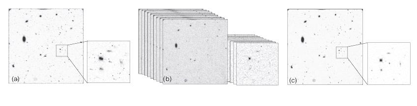
The term DASH (“drift-and-shift”, Momcheva et al., 2016) was adopted to describe the observing strategy of taking a series of WFC3/IR exposures of many targets within one orbit while the telescope is being guided under gyroscope control, thus avoiding the overhead cost of acquiring a new pair of guide stars for every slew between targets of greater than about 2 arcmin. A WFC3/IR sample sequence comprised of short exposure times was selected to limit image smearing within each time step, and the differential samples in one exposure were later aligned and combined to compensate for the greater drift due to gyroscope control (Figure 7.16). 

The DASH technique was originally designed to allow users to carry out shallow large-scale mosaic observations with the WFC3/IR camera but was later adapted to efficiently observe a collection of bright targets within a field ~1 deg across with WFC3/IR subarray apertures (which have shorter time steps for a given sample sequence) and with WFC3/UVIS subarray apertures. Section 6.11.5 provides discussion of using the DASH mode with WFC3/UVIS observations. Below, we provide a detailed discussion regarding HST guiding and previous considerations for program design. 

A DASH orbit must begin with a guide star acquisition followed by at least one exposure using fine guiding to ensure adequate pointing at the beginning of the orbit. Gyroscope performance in later cycles made it necessary to limit each DASH visit to one orbit and to institute a required minimum amount of time using fine guiding. When DASH was supported, the Orbit Planner in APT would show FGS Pause after the exposure(s) taken with fine guiding. The time between the end of the guide star acquisition (GS Acq) and the FGS Pause was required to be at least 5 minutes in order to provide time to update the gyroscope bias before proceeding with a slew or dropping to gyroscope mode. Therefore, in later cycles the orbit must have begun with more or longer guided exposures than in earlier cycles. Previously, Program Coordinators would work with the Principal Investigator (PI) to see if it was possible to plan orbits to achieve the proposed science that fit the scheduling windows.

In APT, all of the exposures must have been grouped together into a non-interruptible sequence container to confine them to one uninterrupted orbit. When placed in this container, the exposures would be observed without gaps due to Earth occultation or SAA passages. As a further precaution, if subarrays were used, it was recommended that PIs carefully choose the minimum size, and use a series of increasingly large subarrays over the course of the orbit as needed to allow for the accumulating telescope pointing drift. PIs were also advised to consider using the offset pattern that minimizes the length of moves during an orbit; offsets are made with a small angle maneuver (SAM), and the repositioning overheads increase with the offset size of the SAM. Overheads for SAMs of different sizes are shown in Table 10.1. More details on planning DASH observations in APT are presented in WFC3 STAN Issue 23.

Some of the earliest IR DASH observations were made under very stable gyro guiding, e.g. Program 14114 (PI: van Dokkum, Momcheva et al., 2016). The exposures were taken with the full array using the SAMP-SEQ=SPARS25 with NSAMP=10, 11, or 12, with 8 sample sequences per orbit. Each sample sequence had 9 to 11 differential exposures of 25 sec, and after dropping to gyro mode the drift in each 25 second interval was on average less than half of a WFC3/IR pixel. The pattern of SAMs resulted in overheads ~1 minute. Suitable step sizes in the WFC3/IR sample sequence depended on the expected accuracy of gyroscope guiding, which has changed with time. When preparing the phase II proposal for a program using DASH mode, it was advised that PIs consult with their Contact Scientist to determine short enough step sizes to mitigate smearing.

The WFC3 team released a set of tools in a DASH pipeline (WFC3 ISR 2021-02; STAN issue 34). Although they are no longer actively maintained, these tools, along with a Jupyter notebook tutorial, remain available through GitHub to assist users with calibrating and reducing WFC3/IR DASH observations.