6.9 Charge Transfer Efficiency
The charge transfer efficiency (CTE) of the UVIS detector has been steadily declining since its installation in 2009 on board HST. Faint sources in particular can suffer large flux losses or even be lost entirely if observations are not planned carefully. In this section, we describe the effect of CTE losses on data, observational strategies for minimizing losses, and data analysis techniques that can provide some correction for CTE losses.
| For the latest information about CTE on the UVIS detector, see the WFC3 CTE webpage. |
6.9.1 Overview
The regular surge of energetic protons and electrons that HST encounters in its frequent passages through the South Atlantic Anomaly results in progressive damage to the silicon lattice of its CCD detectors. This damage manifests as an increase in the number of hot pixels, an increase in the overall dark current, and an increase in the population of charge traps.
The effect of hot pixels, about 1000 new/day/chip using a threshold of 54e–/hr/pix, is addressed with anneal procedures, dark calibration files, and dithering. The anneal procedures, which are performed monthly, warm the detectors to +20° C and restore some of the hot pixels to their nominal dark current levels. Dark calibration files (running averages of daily dark images) can provide reasonable identification of hot pixels as well as a calibration for overall dark current (see Section 5.4.8). The calibration darks allow stable hot pixels and dark current to be subtracted from science images in the calibration pipeline. Since not all hot pixels are stable, the corrections are imperfect, but dithering can help reduce any residual impact of hot pixels in final image stacks.
The effect of charge traps is more difficult to address, as the damage to the detector is cumulative and appears irreversible. The traps prevent photo-electrons from moving perfectly from pixel to pixel during readout. This causes a loss in flux from sources, as well as a systematic shift in the source centroid as some of its charge is trapped and then slowly released during the readout process. The majority of the trapped charge is released within a half-dozen pixel parallel shifts, as can be readily seen in the visible charge trails that follow hot pixels, cosmic rays, and bright stars. A low percentage of the initial signal can be seen extending out to ~50 pixels in length (see Figure 6.22).
Figure 6.22: Residual Charge in Pixels Trailing Hot Pixels
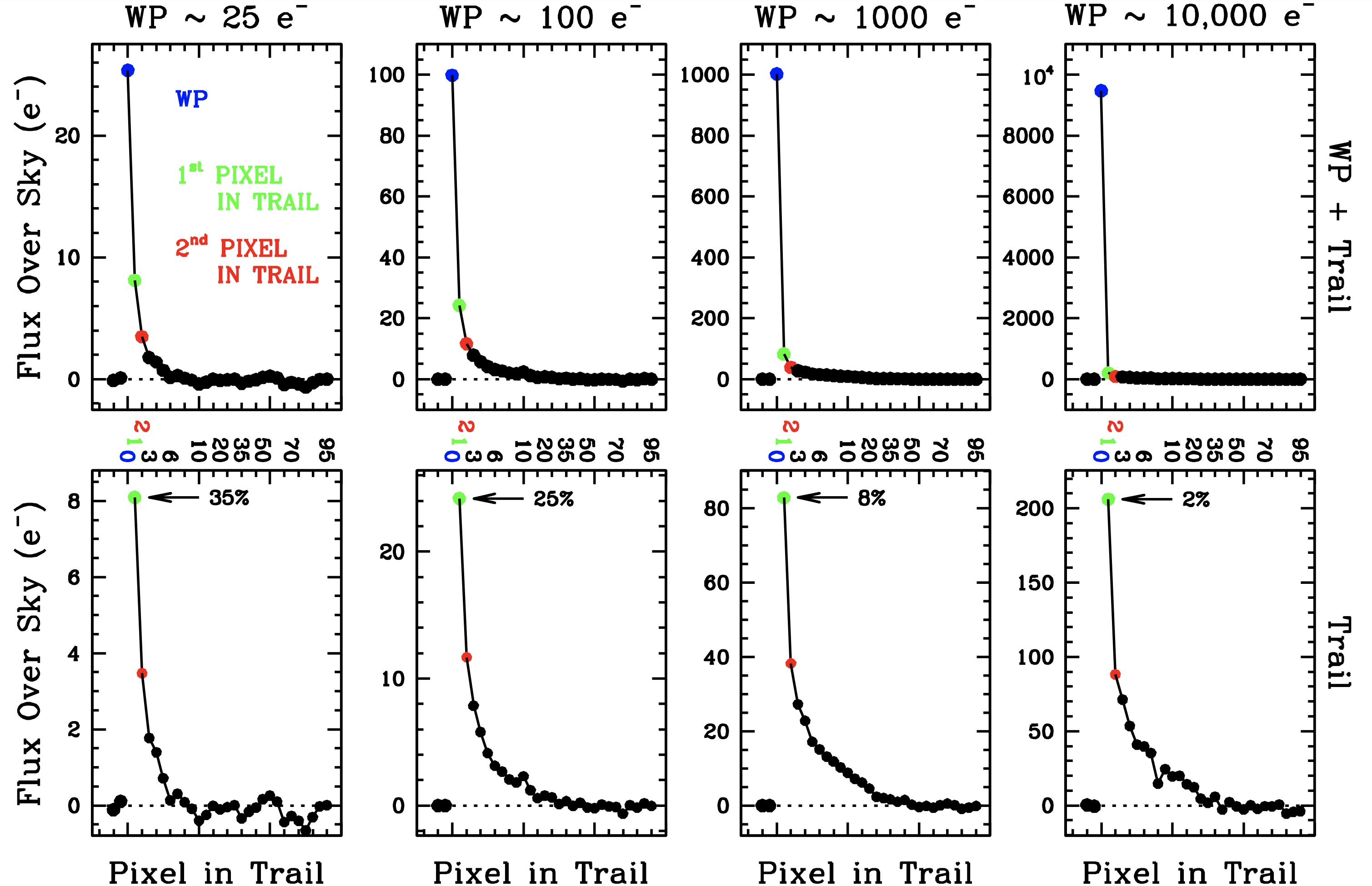
Observed charge trailing far from readout in WFC3/UVIS images with the recommended 20 e- background behind warm/hot pixels (WP) with observed intensities of 20, 100, 1000, and 10,000 electrons in January 2023. These plots give a sense of CTE losses for charge packets of various sizes. The top plot shows the entire range of WP+trail, and the bottom plot zooms in on the trail. The WP on the left started with around 40 e- and by the time of readout, the result is a 25 e- WP and 15 e- in the trail.
- The number of rows between source and readout amplifier: sources farther from the amplifiers (i.e., those closer to the chip gaps) require more parallel transfers before they are read out and thus encounter more traps.
The intrinsic brightness of the source: fainter sources lose proportionally more charge than brighter sources. Very bright sources (those with > 104 electrons) suffer relatively small amounts of CTE loss (a few percent) (see Figure 6.20).
The image background: a higher background keeps many of the charge traps filled, thereby minimizing flux losses during readout of the source signal. WFC3/UVIS images can have very low intrinsic backgrounds due to the low detector readnoise and dark current as well as the small pixels of its CCDs, which subtend less sky. Furthermore, the WFC3 UV and narrowband filters have exceptionally low sky backgrounds. It is when backgrounds are low that CTE losses can become pathological.
- Source size: because of the finite size of the telescope and its optics, point sources do not appear as delta functions on the detector, but rather as point-spread functions with a distribution of pixels above the background. The downstream pixels of a source can shield its upstream pixels from CTE loss by filling some of the charge traps. Resolved objects (galaxies, nebulae, etc.) experience even more self-shielding.
For all these reasons, the impact of imperfect CTE for a particular object will depend on the location and morphology of the source and on the distribution of electrons in the field of view (from sources, background, cosmic rays, and hot pixels). The magnitude of the CTE loss increases continuously as new charge traps form over time. WFC3 ISR 2021-09 provides an overview of our overall current understanding of CTE in WFC3/UVIS, while WFC3 ISR 2024-04 presents updated coefficients for the empirical model for PSF photometry. The CTE website provides an up-to-date list of tools, tips, and insights.
The remainder of this section will discuss the available options for mitigating the impact of CTE losses and their associated costs. Broadly, the options fall into two categories: strategies to implement before data acquisition (i.e., optimizing the observations during the proposal and planning stage, including the use of post-flash if needed), and corrections applied during image analysis after the images have been acquired (i.e., formula- or table-based photometric corrections or pixel-based image reconstruction).
6.9.2 CTE-Loss Mitigation Before Data Acquisition: Observation Planning
1) Consider the placement of the target within the field of view. When the target is small, it can be placed close to a readout amplifier. This reduces the number of parallel transfers during readout, thereby minimizing CTE losses for the target. This can be done by using a subarray aperture (see Figure 6.2); e.g., aperture UVIS2-C1K1C-SUB or UVIS2-C512C-SUB (see Table 6.1) which place the target 512 and 256 pixels, respectively, from the edges of the UVIS detector near amplifier C and read out 1025x1024 and 513x512 science pixels, respectively. (Apertures UVIS2-M1K1C-SUB and UVIS2-M512C-SUB, which place the target closer to the center of the detector, are not suitable for this purpose.) A corollary advantage of subarrays is that many short exposures fit within a single orbit, since only a small portion of the full field of view of the detector is read out and stored.
Alternatively, one can place the target at the reference position of aperture UVIS2-C1K1C-SUB or UVIS2-C512C-SUB, but read out the entire detector instead of only a subarray (aperture names UVIS2-C1K1C-CTE and UVIS2-C512C-CTE, respectively). Full frames can be taken efficiently when the exposures are 348 sec or longer (see Section 10.3.1). Even when a small target is placed near the readout at the bottom of the detector, a full-frame exposure provides more context and enriches the archival value of the exposure. POS-TARGs can also be used to move the target to the lower part of the C quadrant (e.g., negative POS-TARG X and negative POS-TARG Y) to reduce CTE losses even further (See Section 6.4.4 for reasons to prefer quadrant C over the other quadrants).
Another approach, suitable for moderately populated fields, involves obtaining observations at multiple spacecraft roll angles. In this case, the different roll angles (ideally at or near 90 degrees) will result in sources having large variations in the number of pixels over which they must be transferred during readout. This permits a direct assessment of the reliability of the available CTE-correction calibrations that can be applied during post-processing (discussed in more detail below in Section 6.9.3).
If observations are being taken on a field larger than the instantaneous field of view of the cameras, then stepping in the Y direction (i.e., along the CCD columns) with some degree of overlap will place some sources at both small and large distances from the transfer register, thus permitting a direct assessment of the reliability of the CTE corrections applied during data processing (see section on formula/table-based corrections below in Section 6.9.3).
2) Increase the image background. This can be done by lengthening exposure times, using a broader filter, and/or applying an internal background (LED post-flash). Dividing observations into fewer, longer, exposures has several benefits. It provides more natural sky background (thus requiring less post-flash and thereby less added noise), it increases the source signal relative to the readnoise and any added post-flash, and it saves on overheads (each full-frame requires ~90 sec to read out). Ensuring that images with faint sources contain a minimum of 20 e-/pix total background (dark+sky+flash, if needed) is a crucial CTE mitigation strategy for many WFC3/UVIS science proposals in 2020 and beyond (see WFC3 ISR 2020-08). It is worth noting that even higher backgrounds provide more CTE protection; however, more background also produces more noise, so a balance must be struck between preserved signal and added noise. The curves in WFC3 ISR 2021-13 can help with this determination.
On-orbit experimentation has shown that CTE losses are a non-linear function of both the source and image background signals. A faint source in a low-background image will lose a significantly larger proportion of its signal than a similar source in a high-background image. In some cases, faint sources can even disappear completely during the readout transfers, as illustrated in Figure 6.23 below. It is also clear from the curves that CTE affects astrometry as well as photometry: the profiles below are shifted to the right (i.e., away from the readout register), since a star's downstream electrons are more likely to be lost than its upstream electrons.
Figure 6.23: Impact of background on source recovery (epoch late 2020).
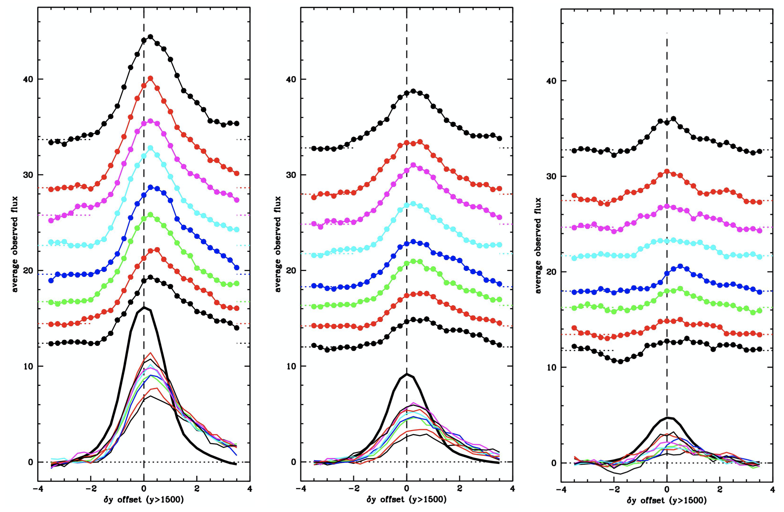
A reproduction of Figure 17 from WFC3 ISR 2021-09. The three panels show three "composite" point sources taken from actual images of real stars with total fluxes of 100 e-, 40 e-, and 16 e-, respectively. The sources were at the top of the detector (2000 pixels from the readout) on eight different image backgrounds ranging from 12 e- to 34 e-. The connected dots show the profiles on top of the various backgrounds, while the curves at the bottom are background-subtracted. The heavy black line shows the true signal expected with no CTE loss. These curves provide a direct sense of the impact that imperfect CTE has on star images.
A more quantitative demonstration of relatively low levels of background significantly improving the CTE and increasing the SNR of very faint sources is provided in Figure 6.24. The background level has a large impact on the photometry of faint sources, but does not have a large effect on bright sources. WFC3 ISR 2021-13 distills many such plots for both photometry and astrometry into tables so that users can anticipate or correct for losses.
Figure 6.24: Quantitative CTE-related photometric losses.
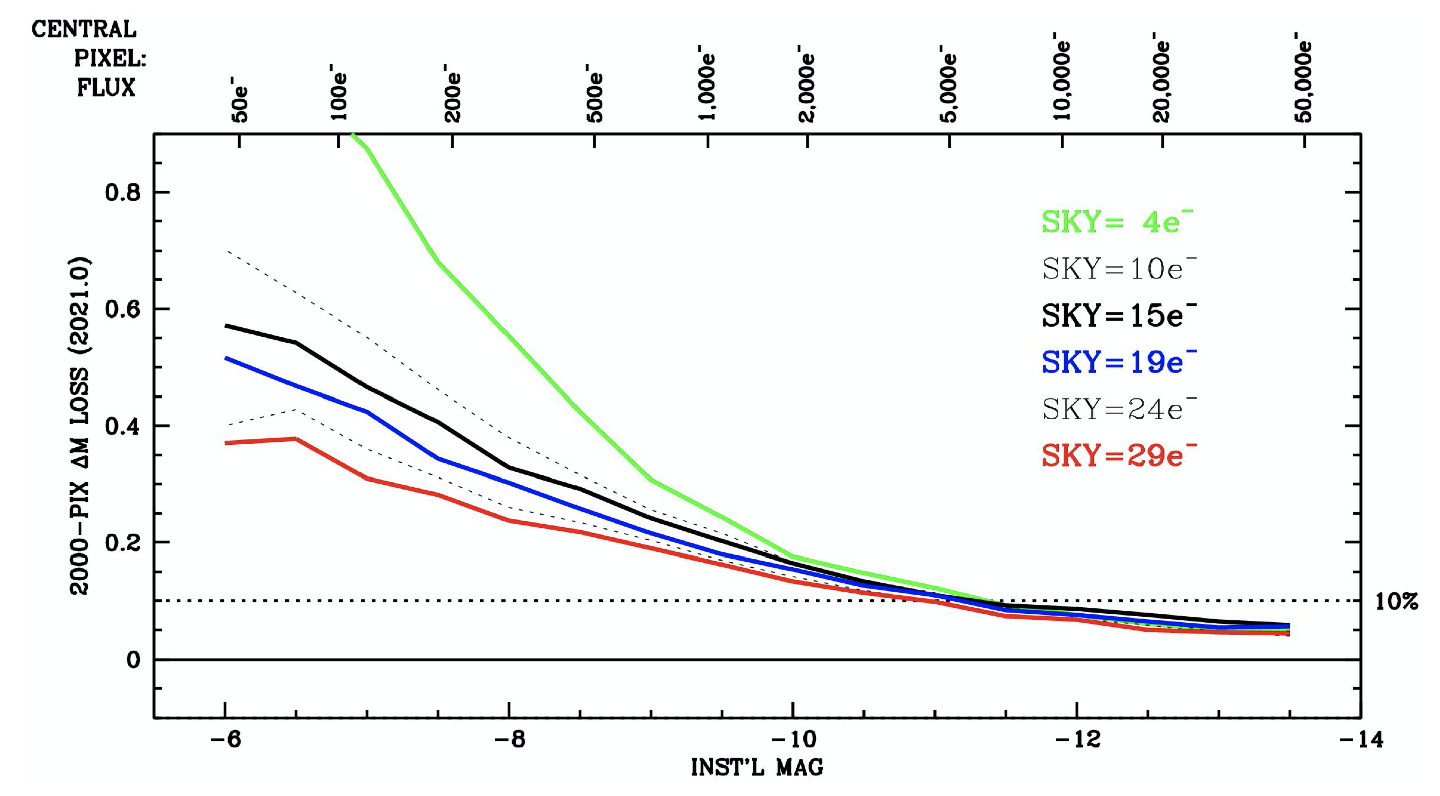
Reproduced from Figure 3 of WFC3 ISR 2021-13. Photometric losses for stars in late 2020 as a function of instrumental magnitude shown for six different backgrounds. Instrumental magnitude is defined as: m = -2.5 log10(flux), where the flux is measured over a 5x5-pixel box and scaled according to a PSF model to correspond to the flux within a 10-pixel radius. The flux in the stars' central pixels are provided along the top of the plot as a reference.
Once users determine the optimal background level for their observations, they need to estimate the natural background to determine how much post-flash to add. The Exposure Time Calculator provides such estimates, including contributions from sky, dark, zodiacal light, earthshine, airglow, and a selected level of post-flash. Alternatively, WFC3 ISR 2012-12 (described above) provides more empirical assessments. In general, if the natural background of the exposure is expected to be higher than 20 e–/pix, then there is usually no need to add post-flash. For images with very low background levels, enough post-flash should be applied to achieve the desired total background (natural + post-flash).
Observers invoke post-flash in APT by choosing the exposure optional parameter ‘FLASH’ and specifying the desired number of electrons per pixel to be added to the image using the LED post-flash lamp. (Section 12.2 in the Phase II Proposal Instructions.) The flash on WFC3 is performed after the shutter has closed at the end of the exposure: an LED is activated to illuminate the side of the shutter blade facing the CCD detector.
On-orbit experience with the LED, corroborated by the design analysis, has shown that although the illumination pattern varies by about +/-20% across the field of view, the pattern is stable and very repeatable (to much better than 1%). The two shutters produce similar though not identical flashes: those on shutter B are ~7% fainter than flashes on shutter A and the ratio of the shutter A/B flash pattern exhibits a smooth ~4% gradient along the diagonal from amplifier D to A (see the "Spatial Dependence of the Flash" section of the WFC3 CTE webpage). Regular monitoring of the post-flash has shown a long term ~0.2%/year decline in the measured counts in both shutter A and B along with apparent random brightness fluctuations from frame to frame of up to +/- 1% (WFC3 ISR 2023, in prep). The long term change is not attributed to the LED but is likely due to the UVIS detector given its consistency with the sensitivity decline measured via photometric monitoring of external targets (WFC3 ISR 2022-04; WFC3 ISR 2021-04).
The post-flash reference files are constructed from stacks of high signal-to-noise post-flash images as a function of shutter blade as well as LED current level setting, normalized to 1 e- per second of flash (WFC3 ISR 2013-12). Prior to 2023, the post-flash reference files were generated from data acquired over ~5 years (WFC3 ISR 2017-13). As of Dec 2022, the post-flash reference files are now time-dependent, generated from data acquired over 1 year time blocks as these provide a slight improvement in data quality (WFC3 ISR 2023-01). All archival data have been reprocessed with the annual post-flash reference files; observers with data retrieved prior to Dec 2022 can re-download their data from MAST to obtain the recent calibration. Note that the default calibration for flashed science images is to remove the flash signal. As a result, the background in the final calibrated pipeline products reflects the astronomical background. To have the pipeline skip the post-flash correction, set the header keyword FLASHCORR to 'OMIT' to turn off the flash subtraction and manually reprocess the data through calwf3.
The main disadvantage of post-flash is, of course, the increase in the background noise. In the worst case, a short exposure with low background and dark current would require the addition of about 20 e–/pix of post-flash. Thus the original readout noise of ~3.1 electrons is effectively increased to 5.4 e– in un-binned exposures. (See Section 9.6 for SNR equations.) In most cases, however, the impact will be significantly less severe, as exposures will generally contain some natural background already and will not require a full 20 e–/pix post-flash. Also, observers can often take fewer exposures, which lessens both the need for and the impact of post-flash.
Finally, please note that even with moderate backgrounds of 20 electrons or more, larger charge packets from brighter stars, hotter pixels, or cosmic rays will still experience some loss/trailing of their initial distribution of electrons. Figure 6.24 shows that even stars near saturation can lose ~5% of their flux to CTE. Therefore, all measurements will require some correction for CTE losses.
3) Use charge injection. This option has been deprecated, but is described here for the sake of completeness. When CTE losses were first addressed, this mode was included as an observing strategy option for CTE-loss mitigation, since the noise penalty from charge injection was significantly lower than Poisson noise of post-flash. However, in practice it is no longer considered to be as useful as optimizing the placement of targets or optimizing the background with exposure times and post-flash. Use of charge-injection will be permitted only in exceptional cases where the science justifies it. Observers who wish to use this mode are advised to consult their Contact Scientist or contact the help desk at http://hsthelp.stsci.edu.
Charge injection is performed by electronically inserting charge as the chip is initialized for the exposure. Charge is injected either into all rows or spaced every 10, 17, or 25 rows. Only the 17-row spacing is supported as of mid-2012. The injected signal is ~15000 electrons (not adjustable) and it results in only ~ 18 electrons of additional noise in the injected rows (Baggett et al. 2011). The rows above or below the charge-injected rows also have between 3 and 7 electrons of added noise due to charge-transfer effects. The charge-injection capability was supported through Cycle 19 (2012), but experience has demonstrated that it is useful for very few types of observations. The primary drawbacks are (1) the noise level in the injected and adjacent rows, (2) the uneven degree of protection from charge trapping in the rows between the injected charge rows, (3) a very difficult calibration challenge posed by the combination of sources in the field and the charge in injected rows, which give rise to different levels of CTE at different places within the image. Furthermore, the strong dependence of CTE losses on image background in the injected images makes it challenging to produce a suitable calibration, as typically there will be a mismatch in image backgrounds between the charge-injection-calibration frames and science frames (i.e., differing levels of CTE losses).
6.9.3 CTE-Loss Mitigation After Data Acquisition: Post-Observation Image Corrections
1) Apply formula/table-based corrections for aperture photometry. One way to correct CTE losses after the images have been acquired is to apply an empirical photometric correction to the measurement via either formulae or tables. The current formula-based results were constructed from stellar aperture photometry, and they provide corrections for CTE losses as a function of observation date, image background, source flux, and source distance from the amplifiers. Figure 6.25 summarizes some of the analysis from WFC3 ISR 2021-03. Plots such as these can be used either to anticipate losses or to correct for them.
As the plots show, larger corrections are required for fainter sources and/or sources observed on lower image backgrounds. The top left panel represents the worst-case scenario: for sources in exposures taken with a narrowband filter, with typically ~2 e–/pix background. Flux losses in early 2023 for sources far from the readout amplifier are ~1 magnitude for the faintest sources measured (a few hundred electrons within a 3-pixel radius aperture). The top right panel shows that a background of ~20-25 e–/pix (~2-12 e– natural plus 10-18 e– post-flash depending on the target) produces a noticeable improvement in CTE: the faintest sources experience about 0.3 mag of losses while moderately bright sources (with a few thousand electrons within a 3-pixel radius aperture) experience less than 0.2 mag of flux loss.
The lower panels in Figure 6.25 illustrate the efficacy of applying the pixel-based CTE correction (discussed in topic 2 below) to the data in the upper panels. Note that these results shown are for small apertures. Corrections for larger apertures will be smaller, as more of the trailed charge will end up getting released within the aperture.
The flux-loss information in these plots has been distilled into formulae, following previous treatments in WFC3 ISR 2015-03, WFC3 ISR 2016-17, and WFC3 ISR 2017-09. In brief, the flux loss is modeled as a function of source brightness, observation date, image-background level, and vertical distance from the readout amplifier and fit with a 2nd-degree polynomial whose coefficients are provided in WFC3 ISR 2021-03 for FLT data, and WFC3 ISR 2021-06 for FLC data, along with the analysis to allow observers to estimate flux corrections for their point-source photometry. The coefficients, as well as other CTE information, can also be found on the WFC3 CTE webpage.
Figure 6.25: CTE Losses in FLT and FLC images as a function of star flux, observation date, and image background level.
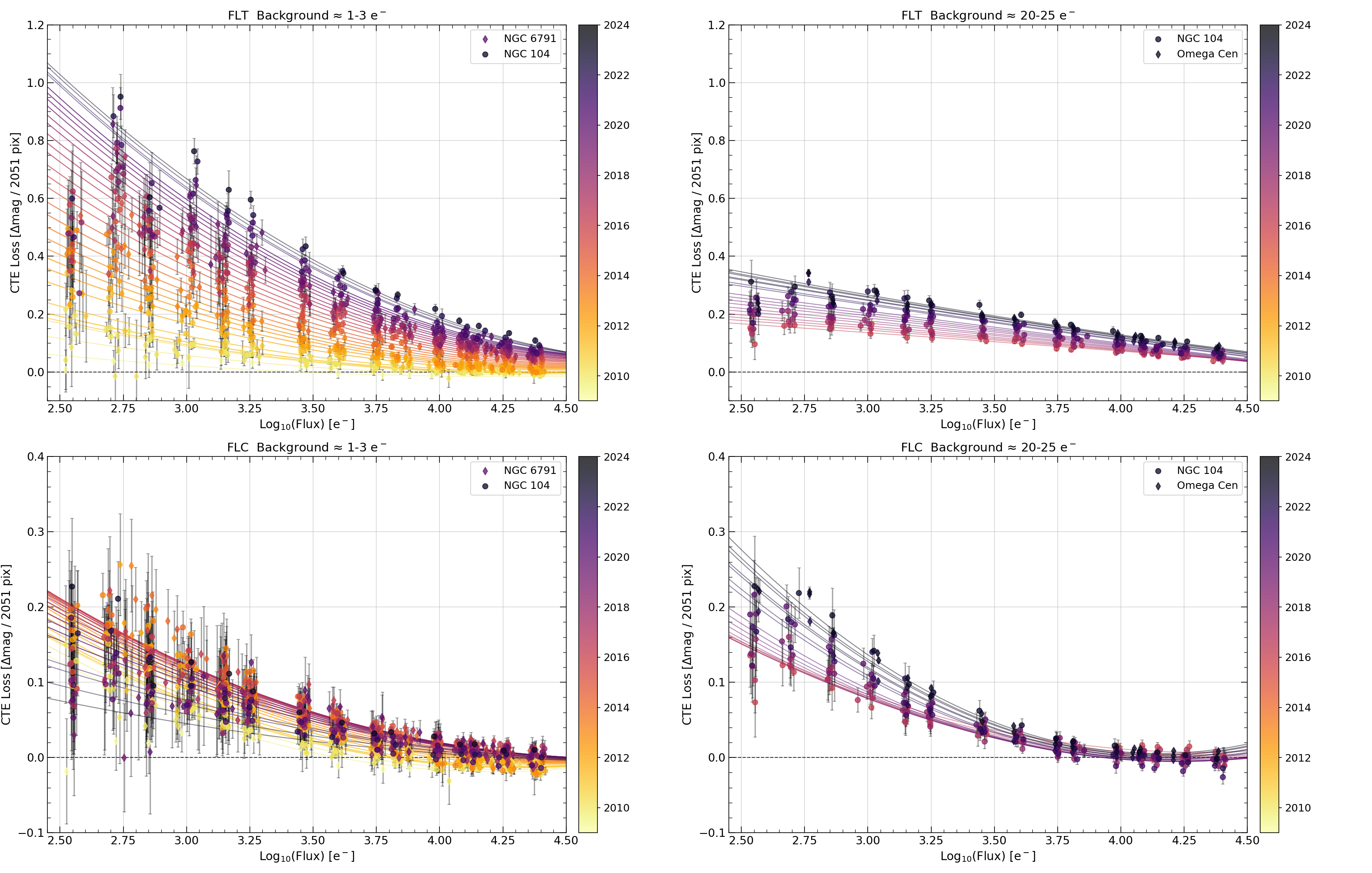
CTE flux losses in magnitudes per 2051 detector-row shifts as a function of star flux (within a 3-pixel radius) and year of observation (color-coded). The top panels show results for data without application of the pixel-based CTE correction (*flt.fits files), low background (~ 2e-/pix) at left and recommended background (~20-25 e-/pix total) at right. Data shown in the bottom row panels have also had the pixel-based CTE correction applied (*flc.fits files). Circular markers are based on NGC 104 (47 Tuc) and diamond markers denote either Omega Centauri or the sparse cluster NGC 6791; lines denote the best fits.
hst1pass, described in WFC3 ISR 2022-05, takes an HST image and produces a list of stars measured in that image. One of the possible outputs of the routine is CTE-corrected photometry and astrometry based on these tables.The formula- and table-based correction approaches can be effective for isolated point sources on flat backgrounds, but they are less suitable for extended sources or sources in crowded regions. However, one benefit of the formula/table-based corrections is that they are not impacted by the possibility of readnoise amplification, which can be a concern for faint sources in the pixel-based reconstruction described below. Photometric corrections are also useful for planning observations: they allow an estimate of the expected CTE losses for point-like sources in a planned observation for a given background and source flux.
2) Apply the empirical pixel-based correction algorithm. The ACS team developed and implemented a post-observation correction algorithm employing the Anderson and Bedin methodology (2010; PASP 122 1035). A similar capability was made available for WFC3, initially in the form of a FORTRAN routine. In Feb 2016, the pixel-based correction was incorporated into calwf3 in the MAST pipeline, which now produces FLC and DRC data products as CTE-corrected versions of FLT and DRZ products. An updated v2.0 version of this correction was made available via the pipeline in 2021 (described in WFC3 ISR 2021-09, performance evaluated in WFC3 ISR 2021-06).
The charge-transfer model is calibrated by studying hot pixels, which serve as delta-function probes of the charge-transfer process. In the absence of CTE losses, the full charge of a hot pixel is entirely contained within a single pixel. If some of the hot pixel charge is trapped due to imperfect CTE, there will be fewer electrons in the hot pixel itself, and more in the trailing pixels (see Figure 6.22). The original charge-transfer model involved examining the trails to determine how many electrons were lost from each original delta-function hot pixel, a strategy that works well as long as the hot pixels suffer moderate fractional losses. To model CTE losses at background/source levels where losses are significant, we devised a strategy of pairing long and short darks to tease out the impact of CTE. The procedure for constraining the model is described in detail in WFC3 ISR 2021-09.
The pixel-based correction algorithm takes the charge-transfer model and uses an iterative forward-modeling procedure. It determines, from the observed distribution of pixel values, what original pixel distribution could be pushed through the CTE-blurring readout simulation to yield the observed pixel distribution. The resulting correction essentially redistributes the counts in the image, “putting the electrons back where they belong” (Anderson et al. 2012).
While the pixel-based algorithm has been successful at removing trails behind stars, cosmic rays, and hot pixels, it has one serious and fundamental limitation: it cannot restore any lost SNR in the image. Faint sources and faint features of extended sources may be so strongly affected by CTE losses that they become undetectable and cannot be recovered (e.g., see Figure 6.23 and Figure 6.24).
Furthermore, the pixel-based reconstruction is essentially a deconvolution algorithm, and as such it can amplify noise or sometimes generate image artifacts. Over the years, CTE losses for faint sources on low backgrounds has become so severe that it is impossible to reconstruct the signal from the faint sources without incurring pathological readnoise amplification. As a general rule of thumb, if CTE losses are greater than 10%, then the reconstruction becomes problematic. If the losses are greater than 25%, then it becomes impossible. The v2.0 algorithm deliberately avoids readnoise amplification, at the expense of leaving faint sources uncorrected. As such, the FLC images should be used to measure only moderate-brightness sources (SNR>10). WFC3 ISR 2021-06 provides a detailed comparison of FLT and FLC photometry against the negligible-CTE-loss case.
The pixel-based correction algorithm also does not correct for sink pixels, which contain anomalously many charge traps (WFC3 ISR 2014-19). They comprise about 0.05% of the UVIS pixels, but can affect up to 1% of the pixels when the background is low. A calibration program to identify sink pixels and pixels impacted by them has been carried out. The strategy for flagging these pixels is presented in WFC3 ISR 2014-22. Since calwf3 version 3.3 was implemented in the pipeline, sink pixels and their trails have been identified in the DQI array with value 1024 (see Table E.3).
Serial CTE trailing (along the X direction on the detector) can be seen in stars, warm pixels, and cosmic rays that are close to saturation. WFC3 ISR 2024-07 provides a comprehensive description of the impact of serial CTE on WFC3/UVIS images. Serial CTE has a much smaller impact than parallel CTE, but it can affect the positions of stars at the scale of 0.01-0.03 pixels. The serial CTE trails drop off much faster than similar parallel trails (the bulk of the trail is concentrated in the first few pixels), but there is an extended low-level tail extending > 1000 pixels. Serial CTE does not have a significant impact on most scientific measurements, but post-pipeline routines are available for users to correct images.
Note that |
We end this CTE Mitigation section by noting that, depending on the science goals, a single mitigation method may not be sufficient for some programs. Observers, particularly those with faint sources, will want to consider applying both pre- and post-observation CTE-loss mitigation strategies. E.g., reduce CTE losses during the readout stage by taking fewer longer exposures to minimize the need for post-flash, but when needed adding post-flash to ensure a background of at least ~20 e–/pix, and then follow that with an application of either the formula/table-based or pixel-based corrections, depending on the nature of their sources. We note that the pixel-based correction algorithms are unable to operate on binned data, even aside from the fact that binning is an ineffective way of increasing the detectability of faint sources that may be impacted by CTE losses (see Section 6.4.4).
For the most current information on the WFC3 CTE and mitigation options, please refer to the WFC3 CTE webpage.
-
WFC3 Instrument Handbook
- • Acknowledgments
- Chapter 1: Introduction to WFC3
- Chapter 2: WFC3 Instrument Description
- Chapter 3: Choosing the Optimum HST Instrument
- Chapter 4: Designing a Phase I WFC3 Proposal
- Chapter 5: WFC3 Detector Characteristics and Performance
-
Chapter 6: UVIS Imaging with WFC3
- • 6.1 WFC3 UVIS Imaging
- • 6.2 Specifying a UVIS Observation
- • 6.3 UVIS Channel Characteristics
- • 6.4 UVIS Field Geometry
- • 6.5 UVIS Spectral Elements
- • 6.6 UVIS Optical Performance
- • 6.7 UVIS Exposure and Readout
- • 6.8 UVIS Sensitivity
- • 6.9 Charge Transfer Efficiency
- • 6.10 Other Considerations for UVIS Imaging
- • 6.11 UVIS Observing Strategies
- Chapter 7: IR Imaging with WFC3
- Chapter 8: Slitless Spectroscopy with WFC3
-
Chapter 9: WFC3 Exposure-Time Calculation
- • 9.1 Overview
- • 9.2 The WFC3 Exposure Time Calculator - ETC
- • 9.3 Calculating Sensitivities from Tabulated Data
- • 9.4 Count Rates: Imaging
- • 9.5 Count Rates: Slitless Spectroscopy
- • 9.6 Estimating Exposure Times
- • 9.7 Sky Background
- • 9.8 Interstellar Extinction
- • 9.9 Exposure-Time Calculation Examples
- Chapter 10: Overheads and Orbit Time Determinations
-
Appendix A: WFC3 Filter Throughputs
- • A.1 Introduction
-
A.2 Throughputs and Signal-to-Noise Ratio Data
- • UVIS F200LP
- • UVIS F218W
- • UVIS F225W
- • UVIS F275W
- • UVIS F280N
- • UVIS F300X
- • UVIS F336W
- • UVIS F343N
- • UVIS F350LP
- • UVIS F373N
- • UVIS F390M
- • UVIS F390W
- • UVIS F395N
- • UVIS F410M
- • UVIS F438W
- • UVIS F467M
- • UVIS F469N
- • UVIS F475W
- • UVIS F475X
- • UVIS F487N
- • UVIS F502N
- • UVIS F547M
- • UVIS F555W
- • UVIS F600LP
- • UVIS F606W
- • UVIS F621M
- • UVIS F625W
- • UVIS F631N
- • UVIS F645N
- • UVIS F656N
- • UVIS F657N
- • UVIS F658N
- • UVIS F665N
- • UVIS F673N
- • UVIS F680N
- • UVIS F689M
- • UVIS F763M
- • UVIS F775W
- • UVIS F814W
- • UVIS F845M
- • UVIS F850LP
- • UVIS F953N
- • UVIS FQ232N
- • UVIS FQ243N
- • UVIS FQ378N
- • UVIS FQ387N
- • UVIS FQ422M
- • UVIS FQ436N
- • UVIS FQ437N
- • UVIS FQ492N
- • UVIS FQ508N
- • UVIS FQ575N
- • UVIS FQ619N
- • UVIS FQ634N
- • UVIS FQ672N
- • UVIS FQ674N
- • UVIS FQ727N
- • UVIS FQ750N
- • UVIS FQ889N
- • UVIS FQ906N
- • UVIS FQ924N
- • UVIS FQ937N
- • IR F098M
- • IR F105W
- • IR F110W
- • IR F125W
- • IR F126N
- • IR F127M
- • IR F128N
- • IR F130N
- • IR F132N
- • IR F139M
- • IR F140W
- • IR F153M
- • IR F160W
- • IR F164N
- • IR F167N
- Appendix B: Geometric Distortion
- Appendix C: Dithering and Mosaicking
- Appendix D: Bright-Object Constraints and Image Persistence
-
Appendix E: Reduction and Calibration of WFC3 Data
- • E.1 Overview
- • E.2 The STScI Reduction and Calibration Pipeline
- • E.3 The SMOV Calibration Plan
- • E.4 The Cycle 17 Calibration Plan
- • E.5 The Cycle 18 Calibration Plan
- • E.6 The Cycle 19 Calibration Plan
- • E.7 The Cycle 20 Calibration Plan
- • E.8 The Cycle 21 Calibration Plan
- • E.9 The Cycle 22 Calibration Plan
- • E.10 The Cycle 23 Calibration Plan
- • E.11 The Cycle 24 Calibration Plan
- • E.12 The Cycle 25 Calibration Plan
- • E.13 The Cycle 26 Calibration Plan
- • E.14 The Cycle 27 Calibration Plan
- • E.15 The Cycle 28 Calibration Plan
- • E.16 The Cycle 29 Calibration Plan
- • E.17 The Cycle 30 Calibration Plan
- • E.18 The Cycle 31 Calibration Plan
- • E.19 The Cycle 32 Calibration Plan
- • E.20 The Cycle 33 Calibration Plan
- • Glossary